Ben Gorman

Ben Gorman

Life's a garden. Dig it.

Challenge

Which digits below represent the number 2?

MNIST samples

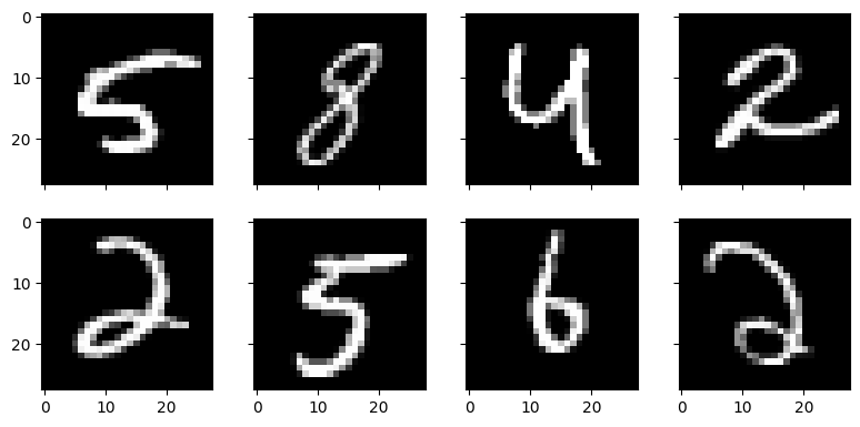
Easy peasy! But can you write a program to classify 2s like these?

In this challenge, your task is to implement a Perceptron to classify handwritten 2s using the famous MNIST dataset. In other words, your model should be able to look at an image and say "this is a two" or "this is not a two".

Data

You can download the MNIST image files from the Kaggle dataset MNIST as PNG. The unzipped file hierarchy looks like this 👇

test/
  0/
    test_image_3.png
    test_image_10.png
    test_image_13.png
    ...
  1/
    test_image_2.png
    test_image_5.png
    test_image_14.png
    ...
  ...
  9/
 
train/
  0/
    train_image_1.png
    train_image_21.png
    train_image_34.png
    ...
  1/
  ...
  9/
 

Every image file is a 28x28 grayscale image of a handwritten digit (0 - 9).

Your job is to make a prediction for each file in test/

Need help getting started?

Here's some code to help you load the data into NumPy array format.

Starter Code
import glob
 
import numpy as np
from PIL import Image
 
# Define constants
TRAINPATH = "/Users/bgorman/Datasets/mnist-png/train"
TESTPATH = "/Users/bgorman/Datasets/mnist-png/test"
 
def load_images(path):
    """
    Given a path, recursively identify all PNG files below the path and load
    them into a list of PIL Images
 
    Args:
        path (str): Directory path like 'pics/mnist/'
 
    Returns:
        tuple(list[Image], list[str]): Returns a 2-element tuple. The first element
        is a list of Image instances. The second is a list of corresponding filenames
    """
 
    images = []
    filepaths = []
 
    for filename in glob.glob(f"{path}/**/*.png"):
        im = Image.open(filename)
        images.append(im)
        filepaths.append(filename)
 
    return images, filepaths
 
# Load the data
trainX, trainFiles = load_images(TRAINPATH)
testX, testFiles = load_images(TESTPATH)
 
# Determine the training data labels
trainY = np.array([file.split("/")[-2] for file in trainFiles])
testY = np.array([file.split("/")[-2] for file in testFiles])
 
# Convert list of Images to arrays with float64 vals
trainX = np.array(trainX, dtype="float64")
testX = np.array(testX, dtype="float64")

Weights and bias

Select the best weights and bias by implementing a guess-and-check algorithm. In other words,

  1. Randomly choose weights and a bias.
  2. Measure the model's performance (accuracy) on the training data.
  3. Repeat this process a few thousand times, keeping track of the best performing weights and bias.

Review the model

Regarding your best model,

  1. Which pixel adds the most evidence that the image represents a 2 as it becomes lighter? Explain why this makes intuitive sense.

  2. Which pixel adds the most evidence that the image represents a 2 as it becomes darker? Explain why this makes intuitive sense.

Solution

import glob
 
import matplotlib.pyplot as plt
import numpy as np
from PIL import Image
 
# Define constants
TRAINPATH = "/Users/bgorman/Datasets/mnist-png/train"
TESTPATH = "/Users/bgorman/Datasets/mnist-png/test"
 
# Random number generator
RNG = np.random.default_rng(2024)
 
def load_images(path):
    """
    Given a path, recursively identify all PNG files below the path and load
    them into a list of PIL Images
 
    Args:
        path (str): Directory path like 'pics/whales/'
 
    Returns:
        tuple(list[Image], list[str]): Returns a 2-element tuple. The first element
        is a list of Image instances. The second is a list of corresponding filenames
    """
 
    images = []
    filepaths = []
 
    for filename in glob.glob(f"{path}/**/*.png"):
        im = Image.open(filename)
        images.append(im)
        filepaths.append(filename)
 
    return images, filepaths
 
 
# Load the data
trainX, trainFiles = load_images(TRAINPATH)
testX, testFiles = load_images(TESTPATH)
 
# Determine the training data labels
trainY = np.array([file.split("/")[-2] for file in trainFiles])
testY = np.array([file.split("/")[-2] for file in testFiles])
 
# Convert list of Images to arrays with float64 vals
trainX = np.array(trainX, dtype="float64")
testX = np.array(testX, dtype="float64")
 
# Standardize the data
trainX = trainX / 255
testX = testX / 255
 
# Declare the model
class Perceptron:
    def __init__(self, w, b):
        self.w = w
        self.b = b
 
    def predict(self, X):
        if X.ndim == 2:
            z = np.sum(X.reshape((1, -1)) * self.w) + self.b
        elif X.ndim == 3:
            z = np.sum(X.reshape((len(X), -1)) * self.w, axis=1) + self.b
        return z >= 0
 
 
# Keep track of the best weights and bias
best = {"accuracy": 0.0, "w": None, "b": None}
 
# Find optimal weights + bias
for i in range(5000):
    if i % 1000 == 0:
        print("Iteration", i)
 
    # Pick random weights and bias
    w = RNG.uniform(-1, 1, size=784)
    b = RNG.uniform(-20, 20)
 
    # Train the Perceptron
    perceptron = Perceptron(w, b)
 
    # Predict on the training data
    preds = perceptron.predict(trainX)
 
    # Measure the accuracy rate
    accuracy = np.mean(preds == (trainY == "2"))
 
    # Check if best
    if accuracy > best["accuracy"]:
        print("New best accuracy:", accuracy)
        best["accuracy"] = accuracy
        best["w"] = w
        best["b"] = b

After 5,000 iterations, the best model classifies 2s with ~91% accuracy on the training data and ~90% accuracy on the test data.

View the output

Iteration 0
New best accuracy: 0.5606166666666667
New best accuracy: 0.82925
New best accuracy: 0.9007
New best accuracy: 0.9007166666666667
New best accuracy: 0.9008
New best accuracy: 0.9014666666666666
New best accuracy: 0.90215
New best accuracy: 0.9054166666666666
Iteration 1000
New best accuracy: 0.9103333333333333
Iteration 2000
Iteration 3000
Iteration 4000
Iteration 5000
Iteration 6000
Iteration 7000
Iteration 8000
Iteration 9000

View the selected weights and bias

print(w.round(3))
# [-0.887  0.006 -0.014  0.592  0.716  0.063 -0.957  0.387 -0.814 -0.565
#   0.613 -0.09   0.032 -0.334  0.568 -0.168 -0.516 -0.748  0.607  0.626
#  -0.615 -0.64  -0.697 -0.767  0.667  0.393  0.564 -0.012  0.804 -0.735
#   0.609  0.53  -0.592 -0.846  0.464 -0.201 -0.327  0.257  0.992 -0.267
#  -0.292  0.329  0.073  0.976  0.843  0.685  0.627 -0.899  0.677  0.873
#  -0.87  -0.2   -0.411 -0.826  0.557  0.781  0.487  0.299 -0.842 -0.144
#   0.454  0.477 -0.136 -0.54   0.34   0.5    0.692  0.737 -0.929  0.102
#  -0.199 -0.063 -0.144 -0.846 -0.619 -0.148 -0.463  0.196 -0.822  0.093
#  -0.678  0.397  0.809 -0.04  -0.451 -0.122  0.341  0.6   -0.322 -0.767
#   0.482  0.252 -0.801 -0.82  -0.063  0.136 -0.219  0.537 -0.996  0.968
#   0.243  0.175  0.543 -0.766  0.261 -0.168  0.933 -0.112  0.172  0.089
#   0.983 -0.782  0.876  0.612  0.294 -0.165 -0.443 -0.142  0.064  0.817
#  -0.444  0.206 -0.66  -0.641 -0.215 -0.425 -0.612 -0.373 -0.693 -0.635
#   0.896  0.55  -0.348 -0.2    0.931  0.937 -0.087  0.566 -0.302  0.012
#   0.542 -0.296  0.436 -0.347  0.562 -0.051  0.221 -0.976 -0.581 -0.061
#   0.899  0.512 -0.778  0.279 -0.032  0.252 -0.342  0.737 -0.539 -0.499
#   0.667  0.126 -0.624  0.325 -0.188 -0.938 -0.466 -0.476 -0.635 -0.45
#  -0.796 -0.301 -0.18   0.964 -0.524  0.419 -0.527  0.638 -0.277 -0.667
#  -0.978 -0.753 -0.816 -0.744 -0.713 -0.354  0.246  0.723  0.012  0.868
#   0.776 -0.81   0.909  0.984 -0.168  0.401  0.082  0.576  0.217  0.865
#  -0.671  0.34   0.026  0.424 -0.068 -0.046 -0.471 -0.577 -0.37   0.897
#   0.944 -0.3    0.7   -0.556 -0.113 -0.491  0.937 -0.802 -0.582 -0.917
#   0.362  0.711  0.614  0.155  0.874  0.203  0.056  0.332 -0.373 -0.937
#   0.589 -0.646 -0.836  0.477  0.546  0.251 -0.575  0.729 -0.182 -0.516
#  -0.086 -0.118  0.421 -0.011 -0.711  0.536 -0.371 -0.184  0.257 -0.094
#   0.331 -0.117  0.095  0.208  0.9    0.635 -0.864 -0.643  0.622 -0.329
#  -0.385 -0.64   0.804  0.24   0.573 -0.319  0.243 -0.461 -0.16  -0.373
#  -0.915  0.168  0.142  0.035  0.217  0.851 -0.455 -0.173  0.56  -0.135
#  -0.116  0.518  0.915  0.602 -0.053  0.7    0.828 -0.614 -0.274  0.31
#   0.486  0.232 -0.623 -0.055  0.243 -0.126  0.341  0.609 -0.235 -0.849
#   0.457  0.263 -0.337 -0.708 -0.599  0.355 -0.079 -0.098  0.223 -0.612
#   0.806 -0.026 -0.42  -0.182 -0.45  -0.923 -0.424  0.722 -0.315 -0.268
#   0.625 -0.61   0.38  -0.876 -0.924  0.263 -0.822 -0.291 -0.774 -0.53
#  -0.012  0.444 -0.498 -0.83  -0.407  0.379  0.463  0.213 -0.536  0.997
#  -0.618 -0.306 -0.989  0.818 -0.523 -0.478  0.576  0.99  -0.772  0.077
#   0.373 -0.054 -0.553 -0.063 -0.903  0.521  0.069 -0.469  0.786  0.208
#  -0.829  0.495 -0.403  0.209  0.955 -0.773  0.476 -0.248  0.999 -0.865
#   0.391  0.426  0.085  0.27  -0.846  0.89  -0.081 -0.974 -0.515 -0.552
#   0.481 -0.959 -0.503 -0.623  0.88  -0.901 -0.398  0.672 -0.579 -0.169
#  -0.621  0.92  -0.08   0.024  0.881 -0.015  0.237 -0.272  0.286 -0.188
#   0.278  0.636  0.156  0.27   0.882  0.018 -0.969  0.56  -0.734  0.514
#   0.626  0.297  0.776 -0.95  -0.214 -0.538  0.073  0.026 -0.979  0.142
#  -0.129  0.215 -0.735  0.303 -0.636 -0.615  0.951  0.539 -0.878  0.16
#   0.266  0.527  0.218 -0.898 -0.071 -0.706  0.353 -0.057 -0.254 -0.644
#  -0.532  0.019  0.998  0.712  0.358  0.006  0.401 -0.079 -0.956 -0.612
#   0.421  0.7   -0.763  0.111 -0.55   0.653  0.072 -0.629 -0.016 -0.984
#   0.176 -0.646  0.445  0.169  0.213 -0.616 -0.048  0.057 -0.497  0.191
#   0.506 -0.109  0.575 -0.72  -0.065  0.837  0.714 -0.267  0.128  0.976
#   0.226  0.966  0.335  0.797  0.127 -0.674  0.012 -0.903 -0.491  0.153
#   0.905  0.845 -0.46   0.706  0.939  0.576  0.907 -0.477  0.245 -0.72
#   0.889 -0.942  0.797  0.352  0.476 -0.583 -0.235  0.22   0.456 -0.939
#  -0.435 -0.651  0.391  0.878  0.77   0.775 -0.103  0.181  0.823 -0.961
#   0.081  0.307 -0.429 -0.124  0.217  0.259 -0.519  0.072  0.461 -0.839
#   0.25   0.057 -0.788 -0.805  0.063 -0.072  0.372 -0.215  0.428 -0.852
#  -0.393 -0.246 -0.36   0.866 -0.562  0.551 -0.06   0.503  0.823  0.064
#  -0.861 -0.253  0.285 -0.757  0.838  0.924 -0.282  0.682  0.38  -0.157
#   0.326  0.195 -0.612 -0.14  -0.534  0.218  0.378 -0.582  0.21   0.511
#   0.72   0.639  0.971 -0.034  0.274  0.93   0.519 -0.919 -0.202 -0.252
#  -0.972 -0.258  0.905 -0.649 -0.752 -0.295  0.744 -0.188  0.795  0.524
#  -0.384  0.109 -0.974 -0.959 -0.065 -0.948 -0.01   0.797 -0.844 -0.15
#  -0.411  0.585  0.106  0.662  0.245  0.15  -0.635  0.412  0.291 -0.162
#   0.924  0.057 -0.985 -0.864 -0.04  -0.953 -0.931  0.908  0.701  0.195
#   0.921  0.08  -0.356 -0.919  0.652 -0.862 -0.221 -0.859 -0.379  0.746
#   0.434 -0.443 -0.903 -0.85   0.236 -0.629  0.787  0.085 -0.062  1.
#  -0.659 -0.772 -0.704 -0.828  0.153  0.979  0.002 -0.676 -0.223  0.141
#  -0.782 -0.561 -0.337  0.811 -0.888  0.109  0.269 -0.862  0.184  0.508
#   0.219  0.434  0.954 -0.869  0.954  0.643  0.662 -0.933  0.618  0.485
#   0.097 -0.346 -0.625  0.988 -0.816 -0.217  0.369 -0.058 -0.601  0.482
#   0.091 -0.567  0.299  0.243 -0.964  0.139 -0.433  0.265 -0.468  0.935
#  -0.59  -0.106  0.023  0.585  0.154 -0.597  0.225 -0.887  0.01  -0.631
#   0.677  0.618 -0.605 -0.099 -0.357 -0.412 -0.12  -0.459  0.29  -0.709
#  -0.952 -0.432  0.911  0.309  0.276 -0.666  0.695  0.055 -0.242  0.715
#  -0.7   -0.327  0.94   0.688  0.844 -0.447 -0.058  0.79   0.449  0.072
#   0.427  0.152  0.306 -0.011 -0.363 -0.779  0.136 -0.65  -0.82   0.833
#   0.586  0.415 -0.289 -0.19   0.792  0.996 -0.691 -0.622 -0.866  0.148
#  -0.695  0.326 -0.852  0.423 -0.146  0.831 -0.918 -0.307  0.476 -0.574
#  -0.302 -0.24  -0.925 -0.999 -0.405 -0.45   0.921  0.834 -0.412  0.035
#   0.636 -0.594 -0.735 -0.975  0.112  0.676  0.125 -0.092  0.371  0.442
#   0.752  0.165  0.267  0.927]
 
  print(b)
  # 14.605564462995053

Model Review

We can identify out the most important pixels by finding the index of the positive and negative weights with the greatest magnitude.

print(np.argmax(best['w']))  # 582 ==> (20, 22)
print(np.argmin(best['w']))  # 214 ==> (7, 18)

In this case, the model implies

  • lightening pixel (20, 22) adds the most evidence that the image is a 2
  • darkening pixel (7, 18) adds the most evidence that the image is a 2

Here are some example images with these pixels highlighted by green and red arrows.

Important Pixels

The large positive weight for pixel (20, 22) makes intuitive sense because it locates the trailing tail of the number "2" - a pixel that is rarely activated by other numbers. Pixel (7, 18) appears to have a large negative weight because it's a popular pixel that's activated by many different numbers.