keywords: COVID-19 testing optimization, Pool testing mathematics, Pandemic response strategies, Test positivity rates, Binomial distribution in epidemiology
The town of Arlington repaved Sunset Road and installed new sidewalks all around. The block of Blossom between Sunset and Lennon had been unpaved for years because it was privately owned, but in 2020 the town paved it anyway. The neighborhood seemed much nicer after all the construction was done, but there was just one problem. There were no stop signs at the four-way intersection of Blossom and Sunset.
Jan and his family lived in the house right on the corner, and we lived in the blue house next door. We were watching the cars go by and realized that since there weren't any stop signs, everyone assumed they had the right-of-way no matter which direction they approached the intersection. Sooner or later there would be a huge wreck at the intersection of Blossom and Sunset. It seemed to us that we had two options. The first would be to inform someone in the town planning department about the serious omission. The second was to calculate the probability of a wreck. We chose option two.
We'll use the Poisson Distribution to estimate how often two cars might be in the intersection at the same time, and the Exponential Distribution to calculate the expected time between crashes.
Before we dive into the Poisson distribution, let's first gather some data about the traffic at our intersection.
Time in the Intersection
Using Google Earth we can estimate the width of the intersection to be 24 feet. Assuming that cars in a residential neighborhood go about 25 mph, or 36.67 feet/second then the total time a car is in the intersection is 0.654 seconds. A handy conversion factor is that 60 mph is exactly 88 feet per second. A further simplification is that the car would only need to be in the same half of an intersection as another one, or they'd have a near miss but escape unscathed. This means that the exposed time in the intersection is just 1/3 of a second.
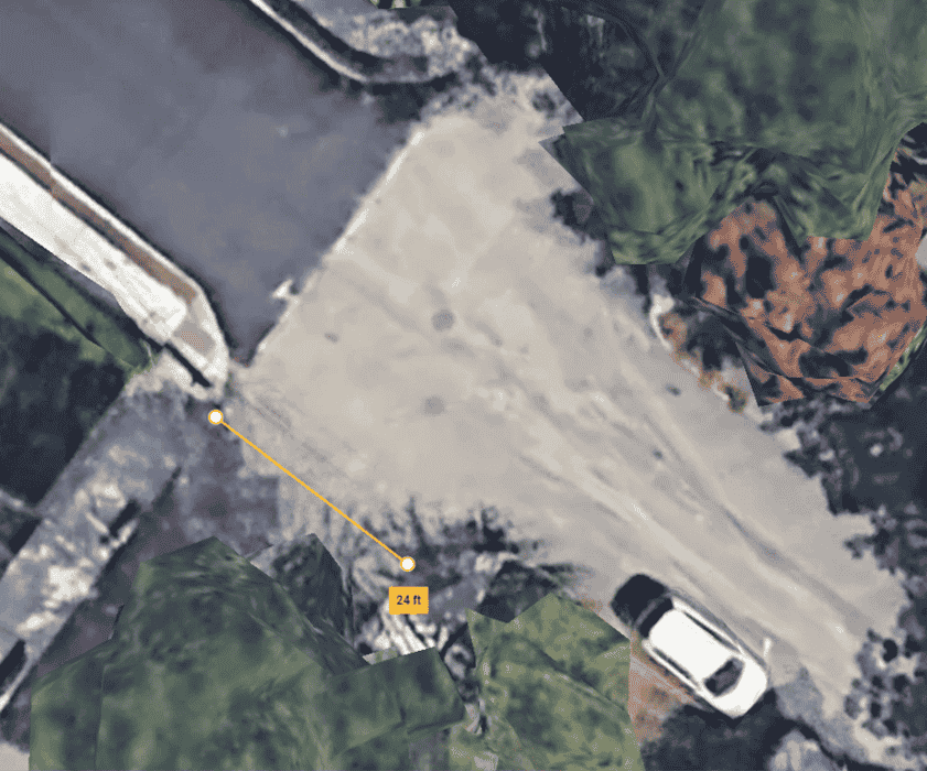
Google Earth view of Blossom and Sunset
I watched the intersection for 95 minutes collecting traffic data and found that 24 cars entered from Blossom and 14 from Sunset. Now that we have our traffic data, we can apply the Poisson distribution to our problem.
Poisson Distributions
To calculate the probability of a wreck, we need to consider the random nature of cars arriving at the intersection. This scenario is well-suited for a statistical tool called the Poisson distribution, which is often used to model the number of events occurring within a fixed interval of time or space, especially when these events happen independently of each other.
The Poisson distribution is particularly useful in situations where we're dealing with rare events - like car crashes - that occur randomly but at a known average rate. In our case, we'll use it to model the arrival of cars at the intersection and, ultimately, to calculate the probability of two cars arriving simultaneously from different directions.
Before we dive into the Poisson distribution, let's first gather some data about the traffic at our intersection.
Letting λ \lambda λ be the average rate events occur, then the Poisson Distribution (video) gives the probability of k k k events occurring in a fixed interval of time, t t t
P ( k events in time t ) = ( λ t ) k e − λ t k ! , P(k \text{ events in time }t)= \frac{(\lambda t)^k e^{-\lambda t}}{k!}, P(k events in time t)=k!(λt)ke−λt,where k ! = k ⋅ ( k − 1 ) ⋅ ( k − 2 ) ⋯ 2 ⋅ 1 k! = k \cdot (k-1) \cdot (k-2) \cdots 2 \cdot 1 k!=k⋅(k−1)⋅(k−2)⋯2⋅1 is k k k factorial. If λ = 2.5 \lambda = 2.5 λ=2.5 then in some time interval t t t, we would expect two and a half events to occur on average. Events are discrete, though, so sometimes it might be that two events happen, and other times three happen. In fact, any non-negative integer number of events might occur, and the distribution (for t = 1 t = 1 t=1) looks like this:
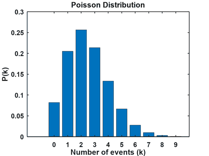
About 25% of the time two events happen, and we'd expect one or three events roughly 20% of the time. There's even a reasonable chance that nothing will happen because the height of the bar for k = 0 k=0 k=0 is about 8%.
We need an estimate for the rate events occur to be able to apply the Poisson distribution. A car passing through the intersection is only exposed for 1/3 of a second, so during the time that I watched the intersection, there were
95 mins × 60 secs min × 3 intervals sec = 17100 intervals. 95 \text{ mins} \times \frac{60 \text{ secs}}{\text{min}} \times \frac{3 \text{ intervals}}{\text{sec}} = 17100 \text{ intervals.} 95 mins×min60 secs×sec3 intervals=17100 intervals.For Blossom, 24 cars entered the intersection so the rate is λ B = 24 / 17100 = 0.00140351 \lambda_B = 24/17100 = 0.00140351 λB=24/17100=0.00140351, and for Sunset the rate is λ S = 14 / 17100 = 0.0008187135. \lambda_S = 14/17100 = 0.0008187135. λS=14/17100=0.0008187135.
If a wreck is going to happen, two events need to occur simultaneously. A car needs to enter the intersection from Blossom at the same moment (1/3 second interval) that a car enters from Sunset. One way of thinking about the rate at which cars enter the intersection is to consider the rate as a probability. So, for Blossom, the probability that a car arrives is 24 observations divided by 17100 1/3-second long intervals. Since we're assuming independence of the events, then the probability of a crash is
λ B × λ S = λ = 24 17100 × 14 17100 = 1.491 × 1 0 − 6 . \lambda_B \times \lambda_S = \lambda = \frac{24}{17100} \times \frac{14}{17100} = 1.491 \times 10^{-6}. λB×λS=λ=1710024×1710014=1.491×10⁻⁶.The 17100 intervals represent 95 minutes of observation, but a more convenient period might be in days. Most of the traffic on Blossom and Sunset happens during daylight hours, usually between 8 AM and 4 PM since there's an elementary school a block away on Blossom. Since there are 8 × 60 = 480 8 \times 60 = 480 8×60=480 minutes in these 8 hours, the number of intervals will be
8 hrs day × 60 min hr × 60 sec min × 3 intervals sec = 86400 intervals day . \frac{8 \text{ hrs}}{\text{day}} \times \frac{60 \text{ min}}{\text{ hr}} \times \frac{60 \text{ sec}}{\text{ min}} \times \frac{3 \text{ intervals}}{\text{ sec}} = 86400 \frac{\text{intervals}}{\text{day}}. day8 hrs× hr60 min× min60 sec× sec3 intervals=86400dayintervals.Now we can estimate the probability of a wreck happening sometime during a day using the formula for the Poisson distribution. The chance of one accident is
P ( k , λ , t ) = P ( 1 , 1.491 × 1 0 − 6 , 86400 ) = 0.09. P(k,\lambda,t) = P(1,1.491 \times 10^{-6}, 86400) = 0.09. P(k,λ,t)=P(1,1.491×10−6,86400)=0.09.Let's call the number of 1/3-second intervals in a day n I = 86400 n_I = 86400 nI=86400. Then the probability of two accidents in the same day is,
P ( 2 , λ , n I t ) = 0.00446. P(2,\lambda,n_I t) = 0.00446. P(2,λ,nIt)=0.00446.Suppose we'd like to know the probability of one or more accidents at the intersection of Blossom and Sunset during the 8 hours. You'd have to sum up all of the probabilities for k = 1 , 2 , 3 , … k = 1,2,3, \dots k=1,2,3,… to infinity.
But, there's an easier way which is to calculate
P ( 0 , λ , n I ) = e − n I λ = 0.9055 P(0,\lambda,n_I) = e^{-n_I \lambda} = 0.9055 P(0,λ,nI)=e−nIλ=0.9055which is the probability that no accidents happen. Then the probability that one or more wrecks occur is 1 − P ( 0 , λ , n I ) = 0.0945. 1 - P(0,\lambda,n_I) = 0.0945. 1−P(0,λ,nI)=0.0945. To calculate the probability of an accident in 10 days, use 1 − P ( 0 , λ , 10 n I ) = 0.629 1 - P(0,\lambda,10 n_I) = 0.629 1−P(0,λ,10nI)=0.629, and in 100 days, 1 − P ( 0 , λ , 100 n I ) = 0.99995. 1 - P(0,\lambda,100 n_I) = 0.99995. 1−P(0,λ,100nI)=0.99995.
Hmmm. Maybe we should have mentioned something to someone.
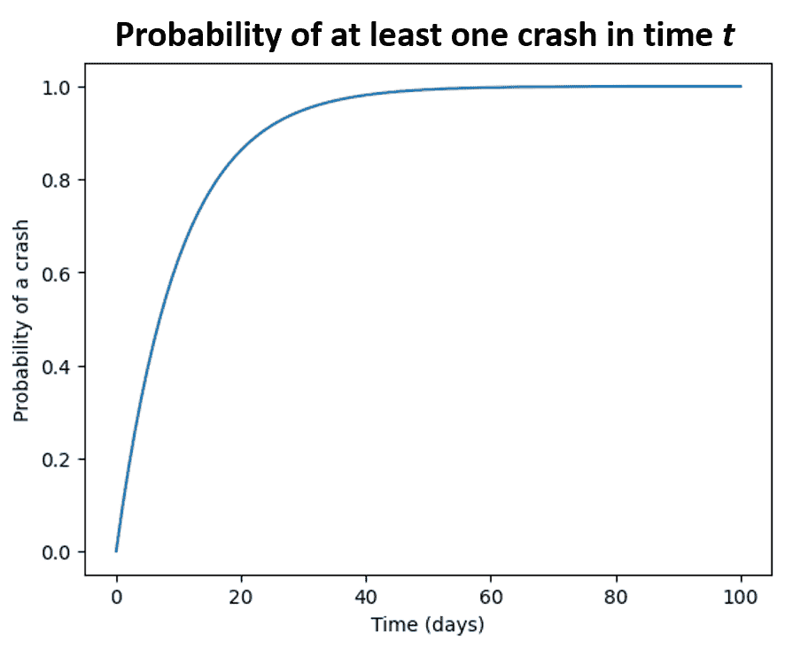
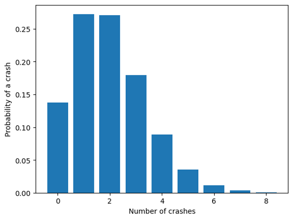
By day 20, the probability of at least one crash is over 80%. A bar chart of the probabilities of 0 - 8 crashes shows the chances of 1 or 2 wrecks to be over 25%, and 3 wrecks is about 18%.
Exponential Distributions
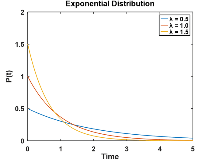
Exponential Distributions complement Poisson Distributions by giving the expected length of time between events. The exponential distribution function is
P ( λ , t ) = { λ e − λ t t ≥ 0 0 t < 0 P(\lambda,t) = \left\{ \begin{array}{ll} \lambda e^{-\lambda t} & t \geq 0 \\ 0 & t < 0 \end{array} \right. P(λ,t)={λe−λt0t≥0t<0which looks like this for several values of the rate parameter λ , \lambda, λ,
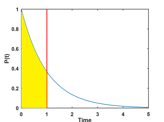
The cumulative exponential distribution is the area beneath the curve up to some time t t t. For λ = 1 \lambda = 1 λ=1 and t = 1 t = 1 t=1, the cumulative distribution is the area shown in yellow here. This area tells you the probability that an event will occur before t = 1. t = 1. t=1. The formula for the area is called the Cumulative Distribution Function (CDF),
C D F ( λ , t ) = 1 − e − λ t . CDF(\lambda,t) = 1 - e^{-\lambda t}. CDF(λ,t)=1−e−λt.
Suppose we'd like to estimate the probability of at least one crash in the next 10 days. It's just
C D F ( λ , n I t ) = 1 − e − λ n I t = 1 − P ( 0 , λ , 10 n I ) = 0.629 CDF(\lambda, n_I t) = 1 - e^{-\lambda n_I t} = 1 - P(0,\lambda,10 n_I) = 0.629 CDF(λ,nIt)=1−e−λnIt=1−P(0,λ,10nI)=0.629showing the relationship between the Poisson Distribution and the Exponential Distribution.
The Intersection of Mathematical Modeling and Reality
So why isn't the intersection of Blossom and Sunset littered with the detritus (Detroitus?) of destroyed automobiles? While our calculations suggest a high probability of crashes at the intersection of Blossom and Sunset, reality hasn't matched our predictions. This discrepancy highlights an important aspect of applied mathematics: models are simplifications of reality and don't always capture every factor at play.
In this case, human behavior and reaction times play a crucial role that our model didn't account for. Drivers, sensing the lack of clear right-of-way, likely approach the intersection more cautiously, reducing their speed and increasing their awareness. This behavior effectively extends the 'safe' time window beyond our calculated 1/3 second, significantly lowering the actual crash risk.
This exercise demonstrates both the power and limitations of mathematical modeling in real-world scenarios. While our model provides valuable insights into potential risks, it also underscores the importance of considering human factors and behavioral adaptations in traffic safety analyses.
The implications of this study extend beyond just one intersection. It raises important questions about urban planning, traffic management, and the balance between mathematical models and real-world observations. How can we better design intersections to naturally encourage safer driving behaviors? How can we improve our models to account for human factors?
For those interested in exploring these concepts further or applying them to intersections in their own neighborhoods, we've provided a JupyterLab notebook. This tool allows you to adjust parameters and calculate crash probabilities for different scenarios. By experimenting with this model, you can gain insights into traffic safety in your own community and perhaps even contribute to local urban planning discussions.
If you'd like to run this experiment for an intersection nearby, install the Anaconda platform and then start the Navigator.

Launch JupyterLab and select the Python kernel. Save a copy of the Blossom_and_Sunset.ipynb notebook locally, and then open it in JupyterLab. You can change the parameters in the notebook to fit your conditions, and then calculate the probability of a crash coming to a neighborhood near you.
So, the next time you approach an unmarked intersection, remember: you're not just a driver, you're part of a complex system of probability and human behavior. Drive safely, and maybe brush up on your Poisson distributions!
Image credits
Hero: Google Street View
Google Earth: Overhead view of Blossom and Sunset
Poisson Distribution video: MathGPT
Anaconda: Anaconda Navigator
Code for this article
The probability of a crash at the intersection of Blossom and Sunset JupyterLab notebook.
References and further reading
- Probability and Statistics by Morris H. DeGroot and Mark J. Schervish - A comprehensive introduction to probability theory and its applications, including the Poisson and Exponential distributions.
- Traffic Flow Theory and Control by D. Gazis - Explores the principles of traffic behavior and their applications to urban planning and accident prevention.
- Poisson Distribution - A detailed explanation of the Poisson distribution, its properties, and applications.
- Exponential Distribution - Overview of the exponential distribution and its relationship with the Poisson process.
- Probability Distribution | Formula, Types, & Examples - In depth article on probability distributions.