California Tumbles Into The Sea

Home

keywords: structure from motion, volume estimation, highway damage, atmospheric rivers, drone mapping

Fire and Rain¶

When he was arrested, Ivan Gomez confessed to five murders and setting the fire to cover up evidence. Police booked him on "charges of arson on forest land, cultivating marijuana, battery on a person, exhibiting a deadly weapon and throwing something at a vehicle intending to cause great bodily injury", but they never found the bodies. His attorney presented evidence that he may not be mentally competent to stand trial, and while the police still believe the origins of the fire were suspicious, they haven't been able to pin an arson charge on him. Firefighters in the area accused him of throwing rocks at their vehicles.

The Dolan Fire on California's central coast near Big Sur began in the evening of August 18th, 2020, and wasn't fully contained until December 31st. Fifteen firefighters were injured battling the fire on September 8th, one of them critically, when they were forced to deploy fire shelters at Nacimiento Station in Los Padres National Forest. By the time the fire was fully contained it had burned 128,050 acres.

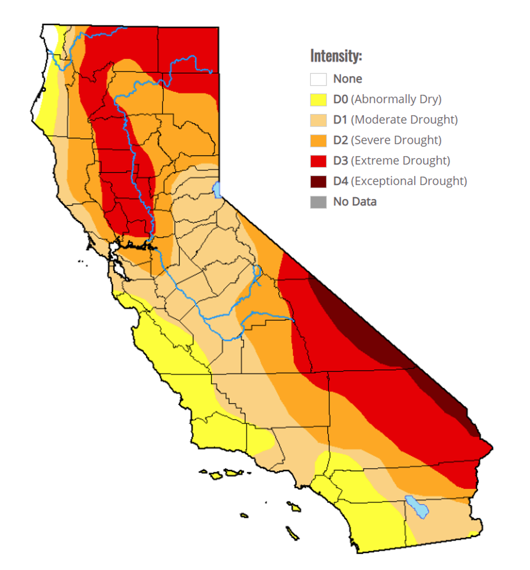
Winter rains of 2020 - 2021 have been only 30% to 70% of the typical totals meaning that groundwater supplies are low. "Northern California remains stuck in one of the worst two-year rainfall deficits seen since the 1849 Gold Rush, increasing the risk of water restrictions and potentially setting up dangerous wildfire conditions next summer", Katherine Gammon writes in The Guardian. Global warming has pushed the start of the fall rainy season back by a month over the past 60 years. The USDA Drought Monitor map for California shows large areas of severe to exceptional drought throughout the state.

Despite persistent dry conditions, one region was about to experience devastating rains. Far out over the Pacific Ocean, an atmospheric river was forming, a "river" in the sky capable of carrying as much water as the Mississippi River. Duane Waliser of NASA’s Jet Propulsion Laboratory says that as the climate warms, atmospheric rivers will increase in intensity. The NOAA page on Atmospheric Rivers (ARs) describes them as mostly beneficial, but when they carry more moisture than normal or stall over a location, ARs can cause significant flooding. In her "Ask Sara" column for Yale Climate Connections, Sara Peach says, "Extreme rainfall from atmospheric rivers is expected to occur more often in the Northwest in the coming decades, and severe winter storms are expected more frequently along the coast."

F. Martin Ralph, director of the Center for Western Water and Weather Extremes (CW3E) at Scripps Institution of Oceanography at UCSD has developed a severity scale for ARs similar to the Safir-Simpson scale for hurricanes. AR Cat1 is weak and primarily beneficial in bringing needed water to snowpacks and other areas, while AR Cat5 is exceptionally hazardous. One example of an AR Cat5 occurred Dec 29, 1996 - Jan 2, 1997 and caused a billion dollars in damage.

On January 27 2021 an AR2 made landfall over the central California coast, moved southward, and stalled near Big Sur. Over the next three days, Big Sur received 13.38 inches of rain, nearly 30% of the annual average. A woman in Monterey County was injured as she attempted to escape a mudslide engulfing her house. Another 24 homes and outbuildings were damaged or destroyed in mudslides caused by the storm. Vegetation burned by the fire meant the ground couldn't absorb much moisture, or withstand the force of the atmospheric river.

A half-hour drive south of Big Sur on Cabrillo Hwy 1 at Rat Creek a torrent of water carrying the burnt remains of trees ripped across the highway washing away a 150-foot long section. California Highway Patrol Officer John Yerace arrived at the scene around 4 PM and was able to stop traffic from entering the area until barricades could be erected.

The San Francisco Chronicle published a review of the events leading up to the washout of Hwy 1 at Rat Creek which included this photo:

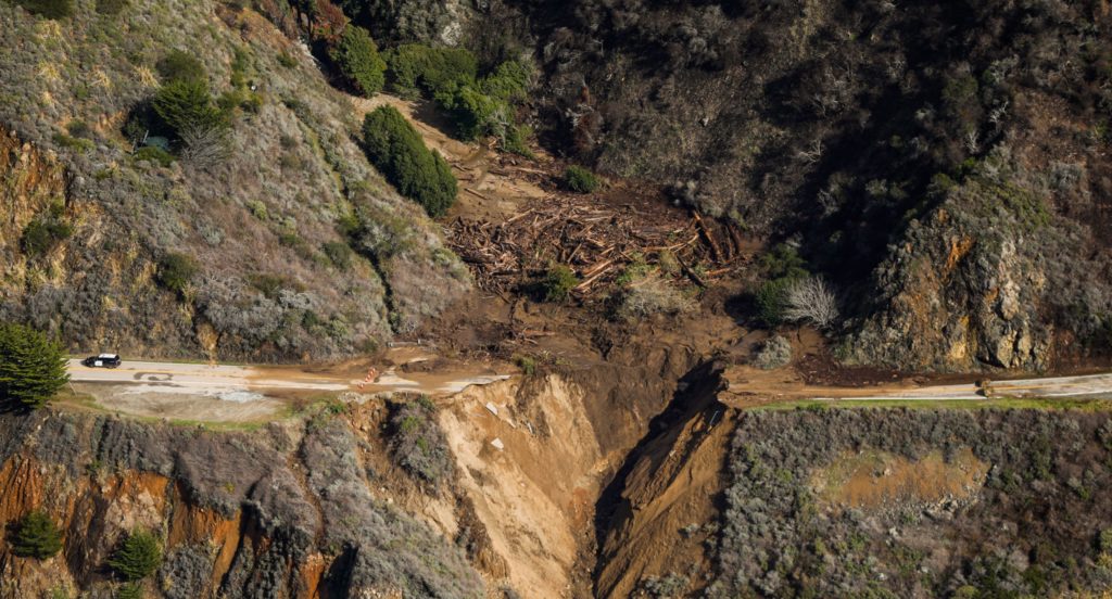
How much of California tumbled into the sea at Rat Creek? This is a question that highway engineers will have to answer as they decide the best approach to repairing the highway. In this case, building a bridge across the chasm may be the best answer, but filling the hole is another possibility and knowing how much fill is required determines the estimated cost.

CalTrans public information officer Kevin Dabrinski said, “It put into perspective my question about, ‘Hey when are you guys going to get this done?’ Because you’re literally standing on a road and you’re looking back up a canyon and there’s marking on the trees about 20 feet up where the mud had risen,” he said. “One of our geotech teams said if we hadn’t had debris flow like if it wasn’t for the debris flow from the Dolan Fire (burn scar), it’s likely that the culvert would have operated as usual and we wouldn’t have had the loss of road.”

Structure From Motion¶

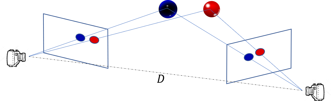
Local news outlets arrived on the scene soon after the washout and flew drones over the area. Even though each video frame is a 2D representation, we can use the combined information from a sequence to reconstruct a 3D model of the washout. With the 3D model, it will be possible to estimate the total volume of the washed-out area.

Structure from motion is a technique of recreating three-dimensional point clouds from a sequence of flat images. The images must have considerable overlap frame-to-frame so that features identified in one frame may be found in subsequent frames. The Scale-Invariant Feature Transform (SIFT) algorithm detects features, and the RANSAC (Random Sample Consensus) method is useful for rejecting non-matching points. Estimating camera pose requires some fairly straightforward linear algebra calculated from the geometry of the locations of points detected in each frame.

San Francisco CBS station KPIX flew a drone over the area capturing video of the damaged highway. During the first 25 seconds, the drone focuses on the washout as the camera moves in a circular arc above the ocean. Beginning at about the 2:45 mark, the drone flies East to West down the valley of Rat Creek with the camera in a nadir pointing attitude. This continues until 3:07 when the drone is above the edge of the ocean and fragments of the highway can be seen in the surf.

This is a clip from a drone flown by ABC7 San Francisco:

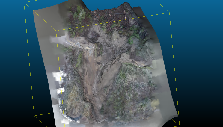
And the view from the Structure from Motion (SfM) 3D reconstruction:

The reconstruction (in .ply format) contains 3.3 million points. Each point is assigned a coordinate (x,y,z) and a color (r,g,b) forming a mesh of triangular patches created from Delaunay triangulation. The video used to make the reconstruction came from the KPIX drone:

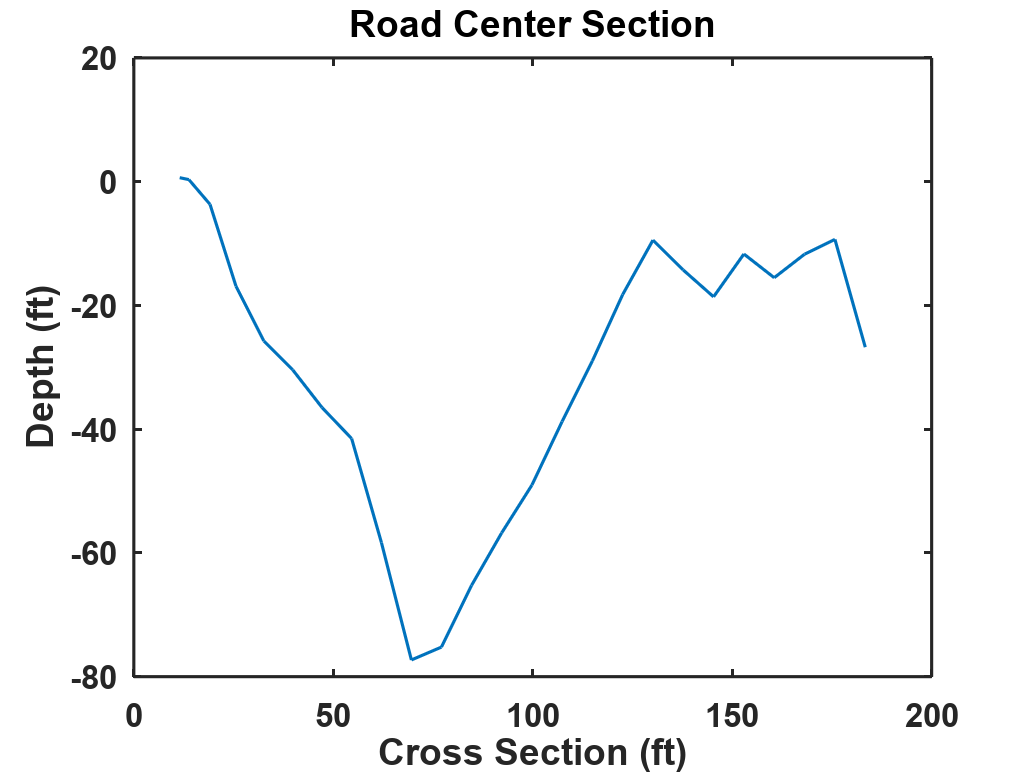
The volume lost directly under the roadway was about 120,000 cubic feet or 4500 cubic yards and a cross-section taken along the centerline of the road shows the maximum depth of the washout to be about 80 feet.

Processing the Data¶

To estimate the volume we first need to get a copy of the drone video and then run it through a Structure from Motion (SfM) tool to get the 3D mesh. Download the drone video using a downloader app such as youtube-dl, and crop the video using Trim Video or Online Converter. I found that the best results were obtained from the sequence 2:45 to 3:06. During this time the drone followed the path of Rat Creek across the road and towards the ocean with the camera pointing straight down.

Several SfM tools are available: AliceVision/Meshroom, Regard3D, VisualSFM, but I found that the online tool VisualSize worked very well. Submit your video clip to PhotoModel3D, provide your email address, and in a couple of hours the completed 3D model is available for download in .ply format, a standard ASCII structure that captures mesh vertex locations and colors. For a very nice 3D model, check out Kathleen Tuite's Sketchfab reconstruction.

Start Google Earth, type "Rat Creek, CA" in the search bar, and click "Search". Next, select a frame from the video that shows a clear view of the damaged roadway, click the "Image Overlay" icon, and import the frame. Set the transparency to about 50% and adjust the size and position of the overlay to match the location.

Using the ruler tool measure the length of the washout and the width of the road. I found the length to be about 148.58 feet and the road width was 21.37 feet. The length matches well with the CalTrans estimate of 150 feet.

Drone video uploaded to YouTube doesn't contain any location data, likely for privacy reasons. Phil Harvey wrote ExifTool to extract header information from video and drones usually include GPS and camera pointing data, but in this case, the data is missing. Aligning an image with Google Earth lets us estimate the scaling and orientation of the image sequence.

Use the mesh processing tool CloudCompare to read the data in the .ply file.

The first step is to take measurements in the 3D mesh and corresponding points in Google Earth. Use the Point Picking tool to select two points that are visible in both the data and Google Earth. Taking the ratio of the distances, I found that the points in the mesh needed to be scaled up by a factor of about 13.947.

Scale the points in the mesh by selecting Edit → Multiply/Scale (make sure "Mesh" is highlighted). If you re-measure the points in the mesh they should match the distances in Google Earth. The scale factor could be improved by taking measurements between several pairs of points and averaging, but we're just trying to estimate the volume of some dirt here.

The SfM tool doesn't have any information about direction, so we need to provide a local reference system. We need to set an $x,y,z$ coordinate system, so I chose the $x$-axis to align with the edge of the road closest to the ocean, and the $z$-axis perpendicular to the road. To align the road with the CloudCompare coordinate system, the first step is to select one point to be the origin $(0,0,0)$. Pick a point on the white line close to the washout area such as point #1 shown here.

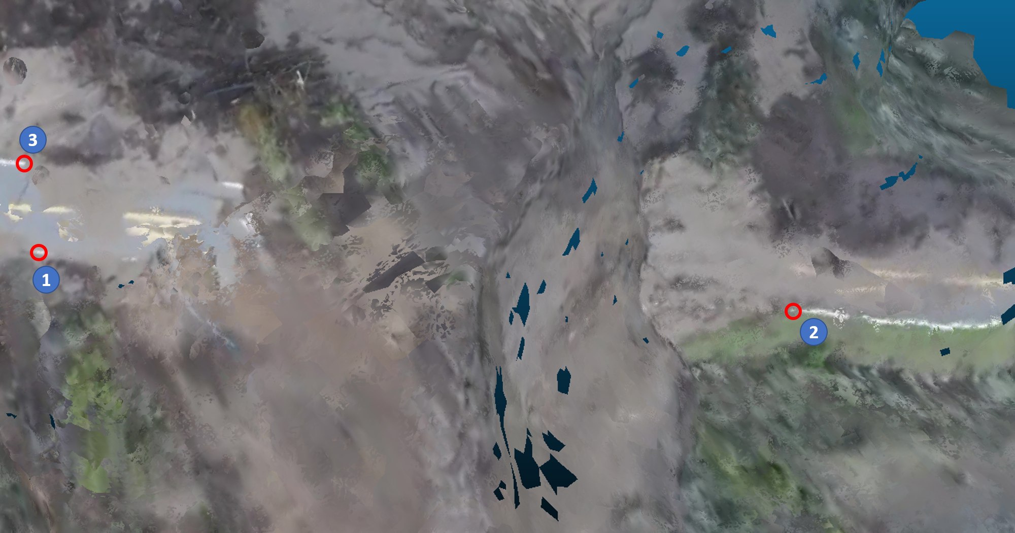
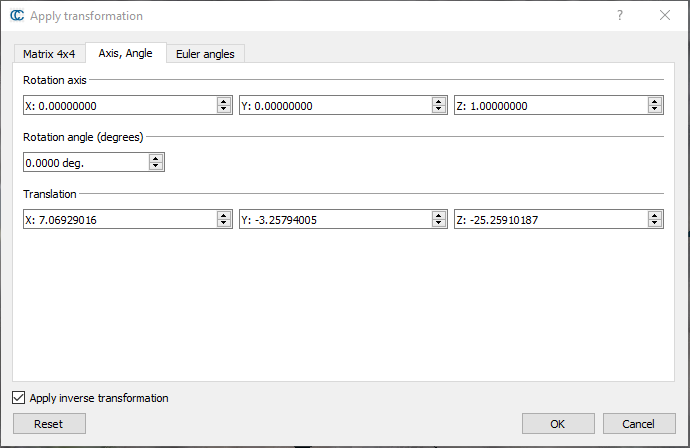
All points will be rotated around this point, so it needs to be close to the opening, but on the edge of the road. Click Edit $\to$ Apply Transformation $\to$ Axis, Angle in the dialog box. Make sure that Rotation axis and Rotation angle values are all set to zero, then enter the coordinates for the first point in Translation, check "Apply inverse transformation" and then OK.

Next, select two more points (2,3), and you should see something like this in the CloudCompare console.

[12:23:42] [Picked] Point@Tri#5421914
[12:23:42] [Picked] - Tri#5421914 (-155.042770;77.017189;-59.749859)
[12:23:42] [Picked] - Color: (194;196;195;254)
[12:23:47] [Picked] Point@Tri#37730
[12:23:47] [Picked] - Tri#37730 (-33.501743;-5.217833;0.409614)
[12:23:47] [Picked] - Color: (233;231;234;255)

Open Octave and load rotationParams.m into the editor. We can now align road points to the CloudCompare axis coordinates. In the Octave command prompt type,

P2 = [-155.042770;77.017189;-59.749859];
P3 = [-33.501743;-5.217833;0.409614];
[omega,theta] = rotationParams(P2,P3,'z')
omega =
 
   0.9909
   0.1345
        0
 
theta = 31.589

Reset the translation values to zeros, and then under "Rotation axis" enter the values from omega: $X:0.9909$ and $Y:0.1345$. The rotation angle is theta $=31.589$ degrees (uncheck "Apply inverse transformation"). Click OK to align the $z$-axis with the local "up" direction. If you use the "Reset" button to clear the form, note that the Z value for the rotation axis is set to 1, not 0. For mathematical details, see the section "Align points to an axis" below.

Once the $z$-axis is aligned with the local up direction, rotate the edge of the road to align with the $x$-axis. Use $P2$ as the first vector, the $x$-axis $[1,0,0]$ as $P3$. The dot product of $P2$ and $P3$ provide the rotation angle

theta = acosd(dot(unit(P2),P3))

Reset the transformation parameters (Ctrl-t) $\to$ Reset and then enter the value calculated for theta as the rotation angle. In this case, the $z$-value should be 1 because we need to rotate about the $z$-axis.

The mesh also needs to be rescaled. The most accurate points are on the white lines along the edge of the road, so pick a point like #3 shown above. The $x$ and $z$ coordinates don't matter, but the $y$ value might be something like 1.532193​. To get the scale factor, divide this into the true road width,

21.37/1.532193
ans = 13.947

In CloudCompare select Tools $\to$ Multiply/Scale, enter the scale factor in Scale(x), and make sure that "Same scale for all dimensions" is checked, then click OK. The $y$-coordinates for points on the white line should now match the road width.

The structure from motion algorithm will miss some points that need to be filled, seen as dark patches. To fill in the missing points, rasterize the point cloud. Use a step size of 0.5, the projection direction z, and for empty cells set "Fill with" to "interpolate". Click "Update Grid" and then "Export Mesh". Highlight the new Vertices field in the DB tree and save it as a newly named file.

The last preprocessing step is to reduce the number of points in the 3D mesh. Import the mesh into Meshlab, then click Filters $\to$ Remeshing, Simplification and Reconstruction $\to$ Delaunay Triangulation, then from the same menu choose Surface Reconstruction: Screened Poisson. This step can be repeated several times until the number of points in the mesh is about 100,000. Save the results as a .ply file. Details of the triangulation process are here.

Calculating the Volume of the Washout¶

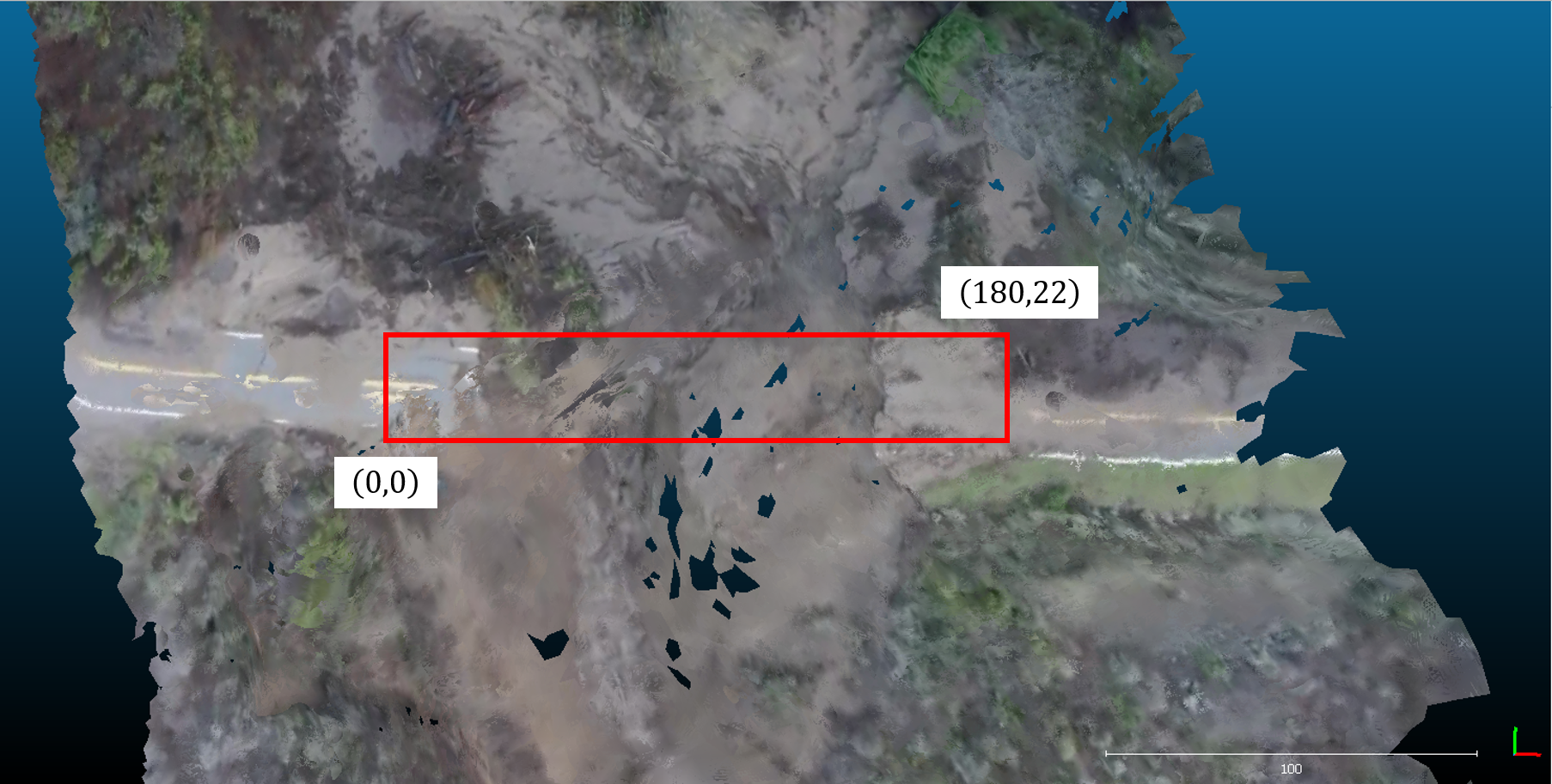
The volume and cross-section functions were written in Octave, and saved to GitHub. Load the .ply file using the function openMesh. This will take a while even with a reduced mesh file. Next, we'll find points in the mesh contained within a rectangle containing the washed-out section of the road. Using CloudCompare, pick a point on the road near Point #2 where the road isn't damaged, and note the $x$-coordinate (about 180 feet). Set the values for upper_right to the length of the section (180 feet) and the known width of the roadway (22 feet).

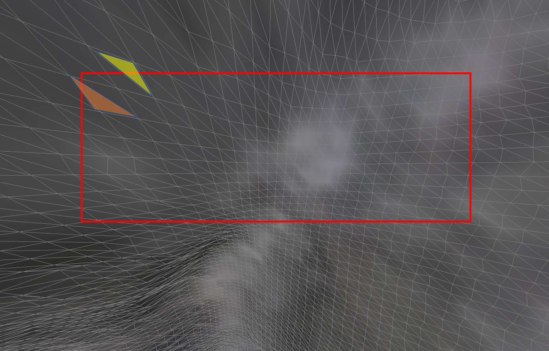
In Octave, the function triInMesh:

lower_left = [0;0];
upper_right = [180;22];
triInRect = triInMesh(mesh,lower_left,upper_right);

returns the indices of all mesh triangles with at least two vertices contained inside the rectangle. In this example, the orange triangle would be counted as inside the rectangle, but the yellow one is outside:

Now the volume under the rectangle can be calculated by summing the volume of each truncated triangular prism:

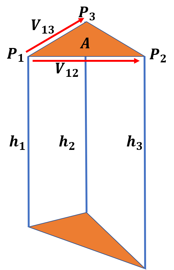
The volume is approximately the area $A$ of the triangle times the height. The height of each vertex $(h_1,h_2,h_3)$ may be different from the others, so an easy estimate is to take the median or middle value. We're just estimating some dirt here. To calculate the area of the triangle first create vectors

and then the area is half the absolute value of the cross product,

In Octave, run the function

meshVol = volUnderRect(mesh,[0;0],[180;22])

to get the volume of the washout under the road. Imagine that you're placing a rectangle over the damaged section of the road where the lower left coordinate is $(0,0)$ and the upper right is $(180,22)$, using a distance down the road of $180$ feet and the road width of $22$ feet. The function volUnderRect calls triInRect as a sub-function, so you don't need to directly find the triangles in the mesh contained within the rectangle.

You can plot a cross-section of the mesh between two points using the function meshCrossSect. The cross-section provides a handy way to check the volume estimate.

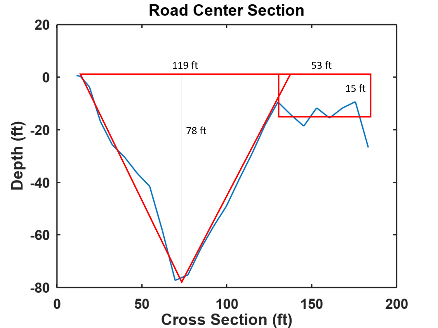
In Octave,

>> (119*78/2 + 53*15)*22
ans = 119592

which is pretty close to the volume estimated using the mesh of $120,330f{t}^3$. The data on the right end is a bit ratty, which may indicate more damage or possibly the road slopes downwards there.

If you want to be useful to CalTrans, they might want an estimate that is slightly wider than the roadway and slopes down away from the shoulders:

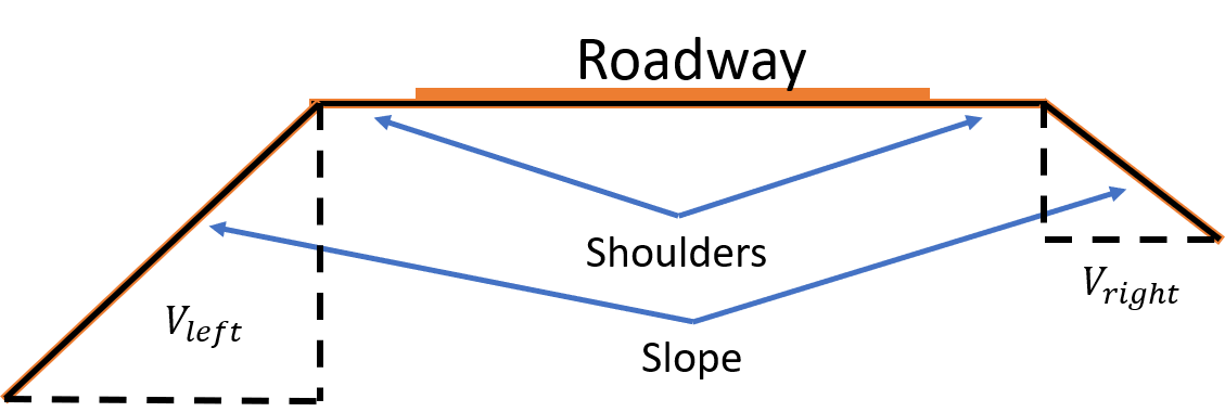
Extending the width of the rectangle by 10 feet on either side to include the shoulders gives a volume of $224320f{t}^3=8308y{d}^3$. If the sloped region is extended 20 feet on either side of the end of the shoulder the volumes are $V_{left}=148,250f{t}^3=5491y{d}^3$ and $V_{right}=79,208f{t}^3=2934y{d}^3$ giving a total fill volume of $V_{total}=451,780f{t}^3=16730y{d}^3$.

Not the end of the road for the Pacific Coast Highway¶

The dramatic events at Rat Creek show that with some open-source software and freely available drone videos it's possible to reconstruct a 3D model of a scene and to perform volumetric calculations. Not only is it relatively fast, but using this technique keeps survey crews at a safe distance from the opening of the washout. Through advanced techniques like Structure from Motion and drone technology, engineers can now reconstruct the affected areas and estimate the volume of the washout with impressive accuracy.

As climate change intensifies weather patterns, the risk of such disasters is likely to increase, highlighting the urgency for innovative solutions in infrastructure resilience. By leveraging tools like drone mapping and 3D modeling, we not only enhance our understanding of these events but also pave the way for more effective responses to future challenges.

Appendix A: Using Your Drone¶

If you own a drone calculations such as these may be easier since GPS data is captured with each frame. First, check that your image data contains GPS using the ExifTool. The blog trek view provides more details on metadata, EXIF, and XMP. Isaac Ullah teaches anthropology at San Diego State University and has posted YouTube videos on constructing 3D point clouds from drone imagery using WebODM, Meshlab, and Grass 7.4, and Basic 3d point cloud analysis in Meshlab, QGIS, and GRASS. OpenDroneMap (ODM) is an "open-source toolkit for processing aerial imagery", able to convert georeferenced imagery into 3D point cloud models. QGIS is an open-source geographic information system (GIS) that integrates other GIS packages including GRASS (Geographic Resources Analysis Support System).

Peter Falkingham recently reviewed SfM generation paths

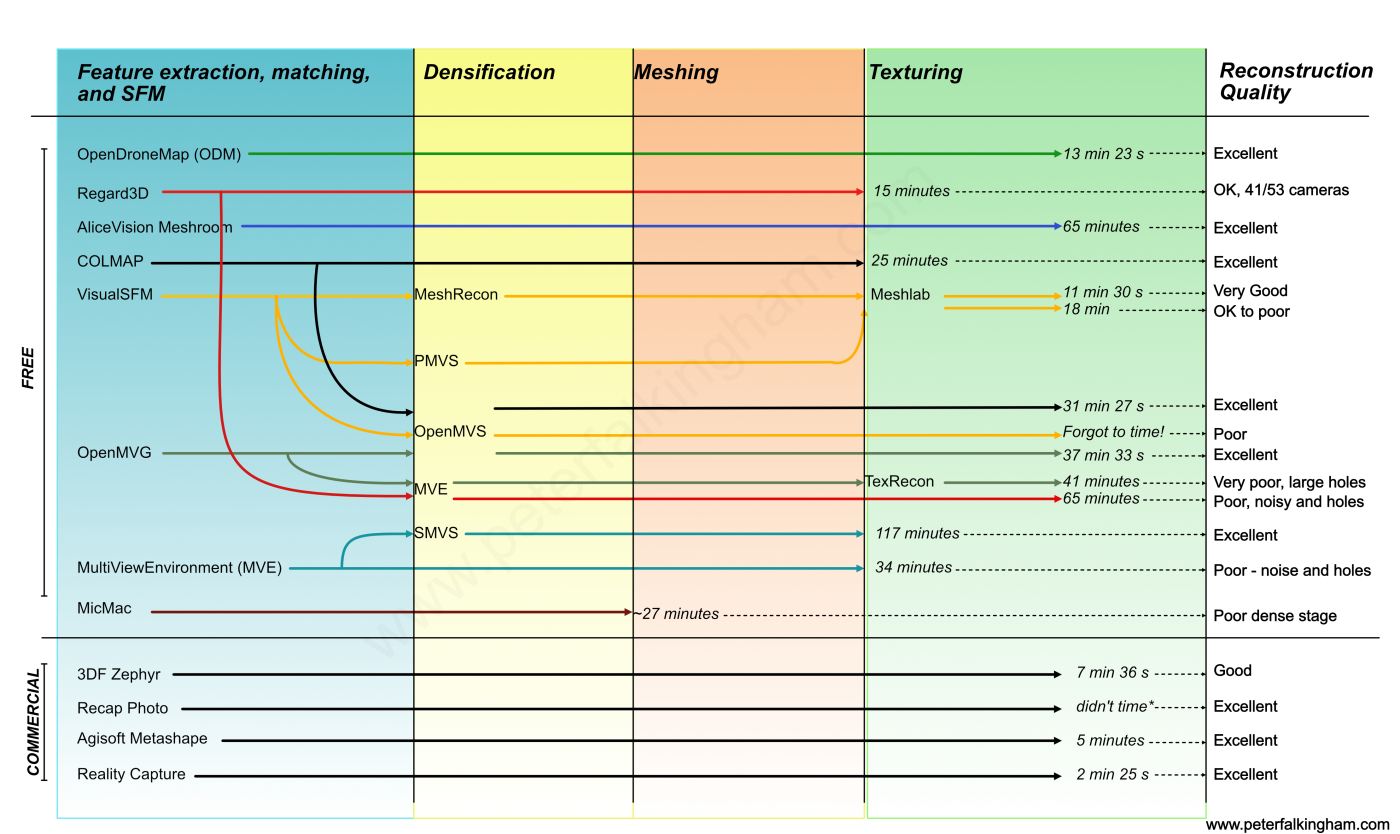
suggesting that OpenDroneMap, AliceVision, and VIsualSFM might be good alternatives to VIsualSize, although VisualSize has the advantage of being entirely online, so no software download is required.

LiDAR may also be used on drones to create elevation point clouds. LiDAR measures distances from the drone to points on the ground by timing a laser pulse transmitted from the drone as the pulse reflects from a point and returns to the sensor. LiDAR only measures distances, so point colors are not available as they are in photogrammetry, but combining LiDAR with data from a camera can restore some sense of color, as Aleks Buczkowski explains in his article, "Drone LiDAR or Photogrammetry? Everything you need to know." Other useful introductory articles are, "Drone photogrammetry vs. LIDAR: what sensor to choose for a given application" and "Should you Choose LiDAR or Photogrammetry for Aerial Drone Surveys?".

Appendix B: Align Points to an Axis¶

The point cloud needs to be rotated to get the direction vertical to the road aligned with the $z$-axis first, then the $x$-axis. As explained above, the first step is to shift all of the points so that the origin is located at a point near the edge of the road just before the washout. Do this by using the translation option and applying an inverse transform equal to the values of this point.

Select two other points, and convert them to unit vectors. A vector is a triplet of numbers describing the direction from one point to another in $(x,y,z)$-coordinates. A unit vector has length $1$, meaning that if $V=[x,y,z]$ then the length of $V$ is $||V||=\sqrt{x^2+y^2+z^2}=1$.

The Octave function norm calculates the length of a vector, so dividing by the norm gives a vector of length $1$, or unit vector. Using these new unit vectors we need to calculate the cross and dot products. The cross product gives a vector perpendicular to the first two, and the dot product is used to calculate the angle between two vectors.

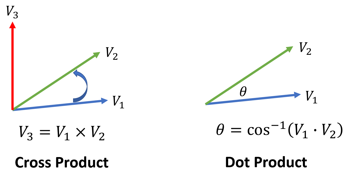
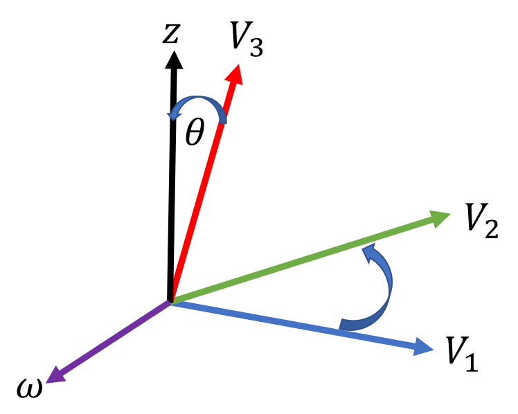
The cross product of $V_1$ and $V_2$ gives $V_3$ which we need to align with the local up direction, or $z$-axis. Taking the cross product of $V_3$ with the $z$-axis $([0,0,1])$ gives a vector perpendicular to both, $\omega$, which is the axis of rotation required to transform all points so that the road becomes horizontal. CloudCompare uses a Rodrigues rotation to rotate points about the origin using information contained in the rotation vector $\omega$ and the rotation angle $\theta$.

After the roadway plane has been aligned with the $x-y$ plane, the edge of the road can be rotated into alignment with the $x$-axis by calculating the angle between them, using the dot product. Pick a point on the white line across the damaged area, but on the same side as the origin, and convert it to a unit vector. The dot product of two vectors is

or the sum of the products of each component of the two vectors. The $x$-axis is the unit vector $[1,0,0]$, so the dot product of any unit vector with the $x$-axis is just the first component of the vector. This means that the angle of rotation required to align to the $x$-axis is

CloudCompare requires the angle to be in degrees, so either multiply by $\frac{180}{\pi }$ or use the Octave function acosd.

Image credits¶

• Hero: Atmospheric river over California, NOAA, Updated March 31, 2023
• The Dolan fire on Sept 8, 2020: Wikipedia, Dolan Fire
• California Drought Feb 11, 2021, U.S. Drought Monitor
• Atmospheric River Science: NOAA, Updated March 31, 2023
• Hwy 1 Washout at Rat Creek: San Francisco Chronicle, Jan. 28, 2021 Stretch of Highway 1 in Monterey County washes away after being hit by debris flow
• Rat Creek Drone Image: San Francisco Chronicle, Jan. 29, 2021 Map: See the part of Highway 1 near Big Sur that fell into the ocean
• Drone Video of Rat Creek Washout: ABC 7 News Bay Area, Drone video shows aftermath of massive landslide on Hwy. 1 near Big Sur
• Drone Video used for SfM Reconstruction: KPIX CBS News Bay Area, RAW: Drone Video Shows Extent Of Washout Damage To State Highway 1
• Google Earth Image Overlay: Google Earth
• CloudCompare Screenshots: CloudCompare 3D point cloud and mesh processing software Open Source Project

Code and Software¶

meshFunctions.m - Octave code to estimate volume from point meshes: openMesh, plyread, rotationParams, triInMesh, knnsearch, meshCrossSect, volUnderRect, volUnderSlope, unit, vnorm, pubFig.

• Meshroom - Meshroom is a free, open-source 3D Reconstruction Software based on the AliceVision framework. To fully utilize Meshroom, a NVIDIA CUDA-enabled GPU is recommended. The binaries are built with CUDA-11 and are compatible with compute capability >= 3.5. Without a supported NVIDIA GPU, only “Draft Meshing” can be used for 3D reconstruction.

• Regard3D - Regard3D is a free and open source structure-from-motion program. It converts photos of an object, taken from different angles, into a 3D model of this object.

• CloudCompare - 3D point cloud and mesh processing software Open Source Project.

• Meshlab - Meshlab, the open source system for processing and editing 3D triangular meshes.

• Octave - GNU Octave is a high-level language, primarily intended for numerical computations.

• Grass GIS - A powerful raster, vector, and geospatial processing engine in a single integrated software suite.

• QGIS - A user friendly Open Source Geographic Information System.

• Google Earth - View high-resolution satellite imagery, explore 3D terrain and buildings, and dive into Street View's 360° perspectives.

See all software used on Wild Peaches →

References and further reading¶

• California wildfires Dolan Fire arson murders mental health evaluation. The Californian, 18 Sep 2020.

• Dolan Fire injuries. KSBY, 8 Sep 2020.

• On atmospheric rivers. Yale Climate Connections, 09 Mar 2019.

• NOAA: What are atmospheric rivers. NOAA, 2018.

• Big Sur Road Collapse. CNN, 30 Jan 2021.

• Rat Creek drone video. KPIX CBS SF Bay Area, 29 Jan 2021.

• Highway 1 Reopen in Big Sur after $11.5 million slide repair. Mercury News, 25 Feb 2021.

📬 Subscribe and stay in the loop. · Email · GitHub · Forum · Facebook

© 2020 – 2025 Jan De Wilde & John Peach