The Kelly Criterion

Home

keywords: Kelly Criterion, Shannon entropy, optimal betting, information theory, Monte Carlo simulation

Two mathematicians from MIT team up with a New Jersey mobster to take down a casino.

Shannon and Kelly at Bell Labs¶

Imagine using a secret formula to win big at blackjack, roulette, and other casino games. That's what two MIT mathematicians, Claude Shannon and John Kelly, Jr., did in the 1950s and 1960s, with the help of a mobster who wanted revenge on the casino owners. In this article, we'll explore how they applied information theory, probability, and the first wearable computer to beat the odds and make a fortune.

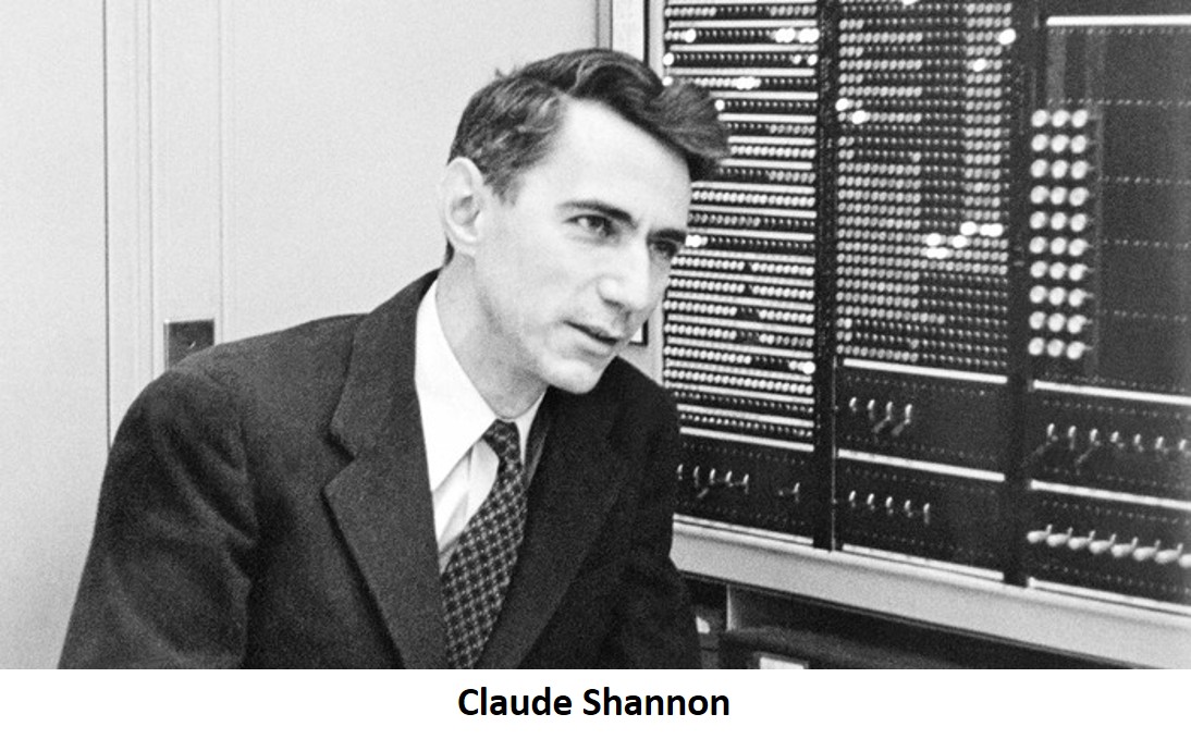
Claude Shannon is known as "the father of information theory" for a paper he published in 1948, "A Mathematical Theory of Communication." For his master's thesis at MIT, he showed that logical operators in electric circuits may by implemented using Boolean algebra. Without these two ideas, the digital information age could not exist.

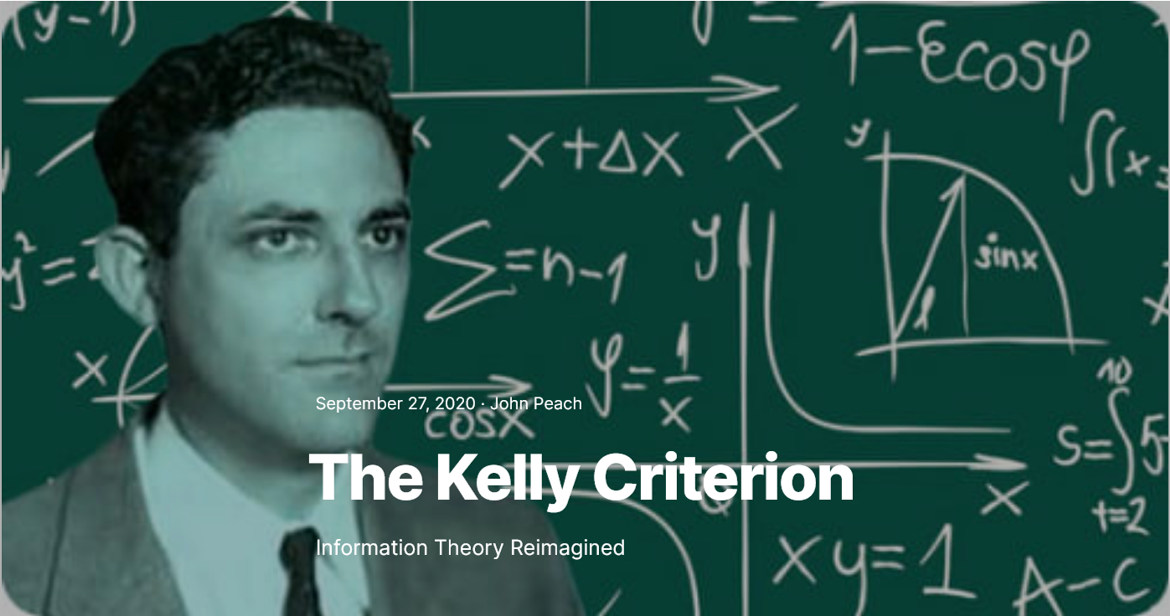
John Kelly, Jr. was a mathematician from Texas who met Shannon when they both worked at AT&T's Bell Labs in Murray Hill, NJ during the 1950s. He read Shannon's paper on information theory and realized it could be applied to gambling. He published his idea in the Bell System Technical Journal in 1956, calling it, "A New Interpretation of Information Rate." Using Shannon's theory, Kelly understood that depending on the probability of winning the bet, you should adjust how big a wager to make.

Information Theory¶

Shannon wanted to know how much information could be transmitted through a channel, where a channel is any form of communication media such as a telephone wire, a transmission from a satellite, or a wink from one spy to another at the ambassador's fancy cocktail party. Shannon considered it from the recipient's point of view, and wondered how much information could be obtained from a message sent through a noisy channel.

He considered it much like a game of Twenty Questions, where one person chooses an object and answers yes or no questions from the other players until one of them can name the object. Shannon wanted to know how many questions on average you might need to ask before you'd know the answer. Let's consider a simplified version where the item is a letter from the set $A,B,C,D$. The best strategy is to first ask, "Is it in the set $\{A,B\}$?". If the answer is yes, next ask if the letter is $A$. If it's not in the set, ask if it's $C$. You'll always get the right answer in two questions if the other player chooses randomly.

Now, let's say you're playing against your young nephew, Abner, who is just learning his alphabet and always carries his stuffed bear toy with him. Little Abner chooses $A$ (for Abner) 50% of the time, $B$ (for Bear) 25%, and splits the other choices $C$ and $D$ evenly at 12.5%. Once you figure this out, your best strategy is to ask if it's $A$ first, then $B$, then $C$. In half the games, you'll be right on the first guess, and in another 25% you'll have $B$ in two guesses. After that, to get $C$ or $D$ will only require one more question. The average number of questions is

$$Q=1\times 0.5+2\times 0.25+3\times 0.25=1.75$$

Shannon derived a formula for this, calling it "Information entropy",

$$H(X)=-\sum _{i=1}^{n}P(x_i){\log }_{2}P(x_i),$$

where $P(x_i)$ is the probability of receiving message $x_i$, and $X$ is the vector of messages, $X=[x_1,x_2,\dots ,x_n]$. You can think of $x_i$ as the letter Abner chooses, $P(x_i)$ is the probability he selects the $i^{th}$ letter, and $H(X)$ is the average number of questions you need to ask him to get the right answer.

Suppose there are $N$ items to choose from, and let's say $N$ is some integer power of $2$. That is,

$$N=2^Q.$$

Because we're playing a yes/no question game, if the item is selected randomly from the set of $N$, then we can split the set in half on the first question, narrow down to a quarter on the second, and so on until we reach the answer. Taking base 2 logs of both sides,

$${\log }_2(N)={\log }_2(2^Q)=Q{\log }_2(2)=Q.$$

Including the probability of selection, and since $\log \left(\frac{1}{x}\right)=-\log (x)$ gives Shannon's entropy equation. In Abner's example,

$$\begin{array}{rl}& H(\{A,B,C,D\})\\ & =-\left[0.5\times {\log }_2(0.5)+0.25\times {\log }_2(0.25)+2\times 0.125\times {\log }_2(0.125)\right]\\ & =-\left[(0.5\times -1)+(0.25\times -2)+2\times (0.125\times -3)\right]\\ & =1.75\end{array}$$

If a gambler has received some inside information he has an edge over the other gamblers. Suppose Aunt Mildred decides to get in on the game with Abner but doesn't realize he favors $A$ and $B$. You somehow convince Aunt Millie to bet on which one of you can get to the right answer first. On average you'll get it in 1.75 while she'll take 2 questions, so you've got an edge. Kelly used Shannon's entropy equation to calculate the optimal amount to bet when you know how much of an edge you have.

The Kelly Criterion¶

There are two extremes to this concept. Most people don't gamble at all and fall into the "nothing ventured, nothing gained" camp. At the other extreme, there are stories of people betting everything they own on red at the roulette wheel in Las Vegas. If you are going to gamble, though, there is an optimal point in between which will give the maximum return.

In the early 1980s before I'd heard about Shannon and Kelly I was thinking about this problem. Using some calculus, I came up with the identical solution that Kelly did. Shannon and Kelly used the mathematics of expectations which provides a rigorous proof, but I like mine because it seems a little more intuitive.

Suppose you have a betting opportunity where there are a series of identical bets. Each bet costs the same amount and the probability of winning is the same each time. For example, you might bet on a coin flip that has a 50-50 chance of paying off if it comes up heads. It costs a penny to play and you win a penny if the coin lands heads. In this case, your expectation is zero since you have to pay a penny to play and you win two pennies half the time, so you're only breaking even. But, maybe you've found an edge and can predict the outcome with better than even odds. How much should you bet each time?

It depends on how much you've brought to the table, and your current stash after playing several games. Let's say you can predict the outcome with probability $p$ and you win $w$ for each penny bet. Suppose you started with $S_0$ dollars initially, and of that, you bet a fraction $b$. Just to get in the game, your stash becomes $S_0-S_{0}b=S_0(1-b)$. If you came with $1 and bet a penny, then you'd be down to 99 cents before the first toss, and if it comes up tails, then that's where you'd be. But, if lands heads, then you win back the fraction you bet times the return $w$, so your stash becomes

$$S=S_0-S_{0}b+S_{0}bw=S_0(1-b+bw).$$

In a long series of these bets, you'll win some and you'll lose some. Let's say you play $n$ times so you'll have a series of wins and losses, {W, L, W, ..., L, W}. Your stash after these $n$ bets will be something like,

$$S_n=S_0(1-b+bw)(1-b)(1-b+bw)\cdots (1-b)(1-b+bw).$$

Of the $n$ bets, you can expect to win $pn$ of them, and lose $(1-p)n$ others. The order doesn't matter since they all get multiplied together, so the amount you win will be $S_0(1-b+bw{)}^{pn}$ and the amount you lose will be $S_0(1-b{)}^{(1-p)n}$. Combining these, your stash becomes

$$S_n=S_0(1-b+bw{)}^{pn}(1-b{)}^{(1-p)n}.$$

If we let $R_n=S_n/S_0$ be the ratio of your initial stash to final stash, this formula becomes

$$R_n=(1-b+bw{)}^{pn}(1-b{)}^{(1-p)n}.$$

Factoring out the $n$ gives the expected return per bet,

$$R=(1-b+bw{)}^p(1-b{)}^{(1-p)}.$$

Recall that $b$ is the fraction of your current stash you bet each time, $0<b<1$. What we'd like to do is maximize $R$ as a function of $b$, which means we need to take the derivative of this equation, set it equal to zero, and solve for $b$. Using the product rule of derivatives,

$$\frac{dR}{db}=\frac{d}{db}u\cdot v=udv+vdu,$$

so letting $u=(1-b+bw{)}^p$ and $v=(1-b{)}^{(1-p)}$ we have

$$du=p(w-1)(1-b+bw{)}^{p-1}$$

and

$$dv=-\frac{(1-p)}{(1-b{)}^p},$$

so

$$\frac{dR}{db}=-(1-b+bw{)}^p\frac{(1-p)}{(1-b{)}^p}+(1-b{)}^{(1-p)}p(w-1)(1-b+bw{)}^{p-1}.$$

It looks complicated, but remember that what we need to do is to set this to $0$ and solve for $b$,

$$-(1-b+bw{)}^p\frac{(1-p)}{(1-b{)}^p}+(1-b{)}^{(1-p)}p(w-1)(1-b+bw{)}^{p-1}=0.$$

First, multiply both sides by $-(1-b{)}^p$ to get

$$(1-b+bw{)}^p(1-p)-(1-b)p(w-1)(1-b+bw{)}^{p-1}=0.$$

Next, multiply both sides by $(1-b+bw{)}^{-p+1}$ which gives

$$(1-b+bw)(1-p)-(1-b)(w-1)p=0.$$

Expanding and collecting terms,

$$\begin{gathered} (b-p)w-b+1=0 \\ bw-pw-b+1=0 \\ b=\frac{pw-1}{w-1}. \end{gathered}$$

If the product $p\times w>1$ you can expect to win in the long run if you use the Kelly optimization. Here's an example where $p=1/2$ and $w=3.$ The Python function to plot this is plotReturnRatio.py.

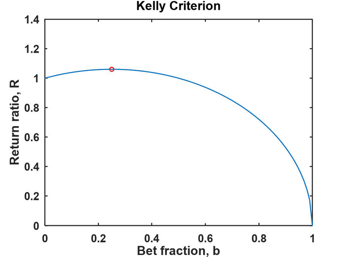
The red dot is where the ratio reaches a maximum and happens when

$$b=\frac{pw-1}{w-1}=\frac{3/2-1}{3-1}=\frac{1}{4}.$$

Putting $b=\frac{1}{4}$ into the function $R(b,p,w)$ gives a maximum return ratio of $R_{max}=1.0607$, meaning your stash will grow at a rate of about 6% per bet. Professor Albert Bartlett has said, "The greatest shortcoming of the human race is our inability to understand the exponential function." He was referring to population growth and energy, but understanding it in terms of how much your pile of money can grow when properly bet might also be important to you. By increasing the size of your next bet after a win and decreasing it after a loss you can achieve exponential growth.

Notice for $b=0$ the return ratio is 1 meaning if you don't play you can't win. At the other end, $b=1$ which is when you gamble everything. Unless the outcome is certain, you'll lose it all sooner or later. For $b=0.5$ the curve has come down to 1 and for all values of $b>0.5,R<1$. Even though you might correctly predict the outcome and have a positive expectation, you can still lose money if you bet too large a fraction of your money.

A Monte Carlo Experiment¶

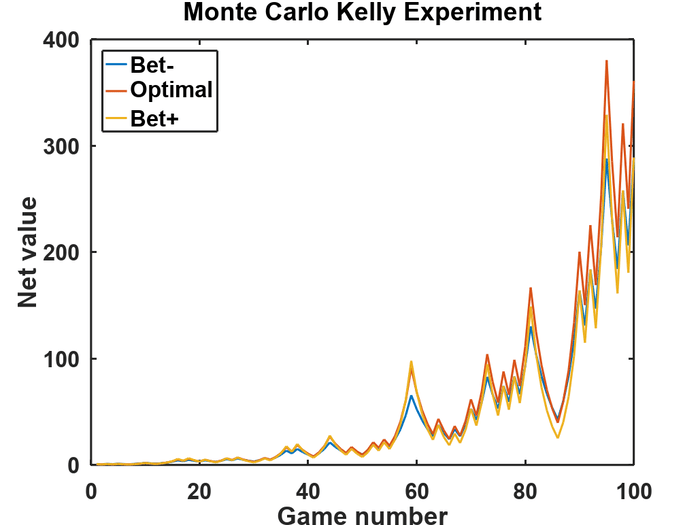
Now that we've derived the Kelly Criterion mathematically, you might be wondering: "Does this actually work in practice?" After all, the real world is messier than pure mathematics. To bridge this gap between theory and reality, let's put the Kelly Criterion to the test.

We can do this through what's called a Monte Carlo experiment - a computational method that uses repeated random sampling to obtain numerical results. Think of it as running thousands of virtual betting scenarios to see if our mathematical predictions hold up. Just as casino operators in Monte Carlo use large numbers of bets to ensure their house edge, we'll use computer simulation to verify our optimal betting strategy.

Here's a Monte Carlo experiment of the Kelly Criterion in which the outcomes of each game are randomly chosen by the computer so it's very much like a real coin toss game. The values for $p$ and $w$ are still the same as before, but each outcome is unknown before the bet. I ran three different cases for the value of $b$. There's the optimal value of $b_{opt}=0.25$ and two other cases, Bet- and Bet+ where $b=b_{opt}\mp 0.05$. At the end of the experiment, the stash for the optimal case is $361.1, but for the other two, it's only $289 starting with an initial amount of just $1. It's a little hard to see because the curves are wiggling around a lot, but there is quite a difference in the outcome.

Breaking the Bank¶

Claude Shannon left Bell Labs to become chairman of the Mathematics Department at MIT. One day a junior faculty member, Ed Thorp, asked Shannon for help getting a paper published.

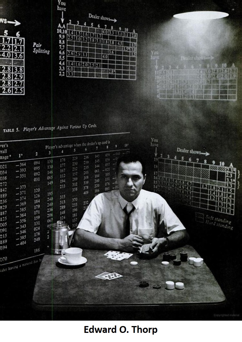
Roger Baldwin, a mathematician working at the Army's Aberdeen Proving Ground in Aberdeen, MD along with three associates, used an Army computer to calculate the odds when playing blackjack. The computer was supposed to calculate the ballistic trajectories of gunnery shells, but they took advantage of downtimes at night and discovered that by playing an optimal game the house odds could be brought down to just 0.62.

Thorp read their paper and realized they had assumed the dealer shuffled after every play. Casinos don't want to slow the game down, so multiple hands are dealt before reshuffling. Thorp recalculated the optimal strategy when the dealer doesn't shuffle which gave the player the edge when the player counts cards.

As a mathematical paper, Thorp's didn't make a big impression. But word got out and news reporters began to call. Gamblers all over the country called to ask for copies of Thorp's paper. Thorp became an instant celebrity. Thorp and Shannon wanted to apply the card counting blackjack scheme along with Kelly's method in a Nevada casino, but they needed front money.

Manny Kimmel, a mobster from Newark, NJ ran a numbers racket. He also held a grudge against the owners of some Reno casinos. Watching Thorp play mock blackjack games, Kimmel became convinced that Thorp could beat the casinos. Kimmel wanted to front Thorp and Shannon $100,000, but Thorp talked him down to $10,000. They flew into Reno one weekend and after about 30 hours of play, they were up to about $21,000 and could have been over $30,000 except that Kimmel was betting on the side and losing.

Shannon and Thorp later built the first wearable computer to beat roulette. John Kelly developed a speech synthesizer while working at Bell Labs, and used it to create the song "Daisy Bell" which Arthur C. Clarke included in the movie "2001: A Space Odyssey". He died of a stroke at age 41 in 1965 and never used his method to make money. Thorp is now president of Edward O. Thorp & Associates where his investments have yielded an average growth of 20% for almost 30 years.

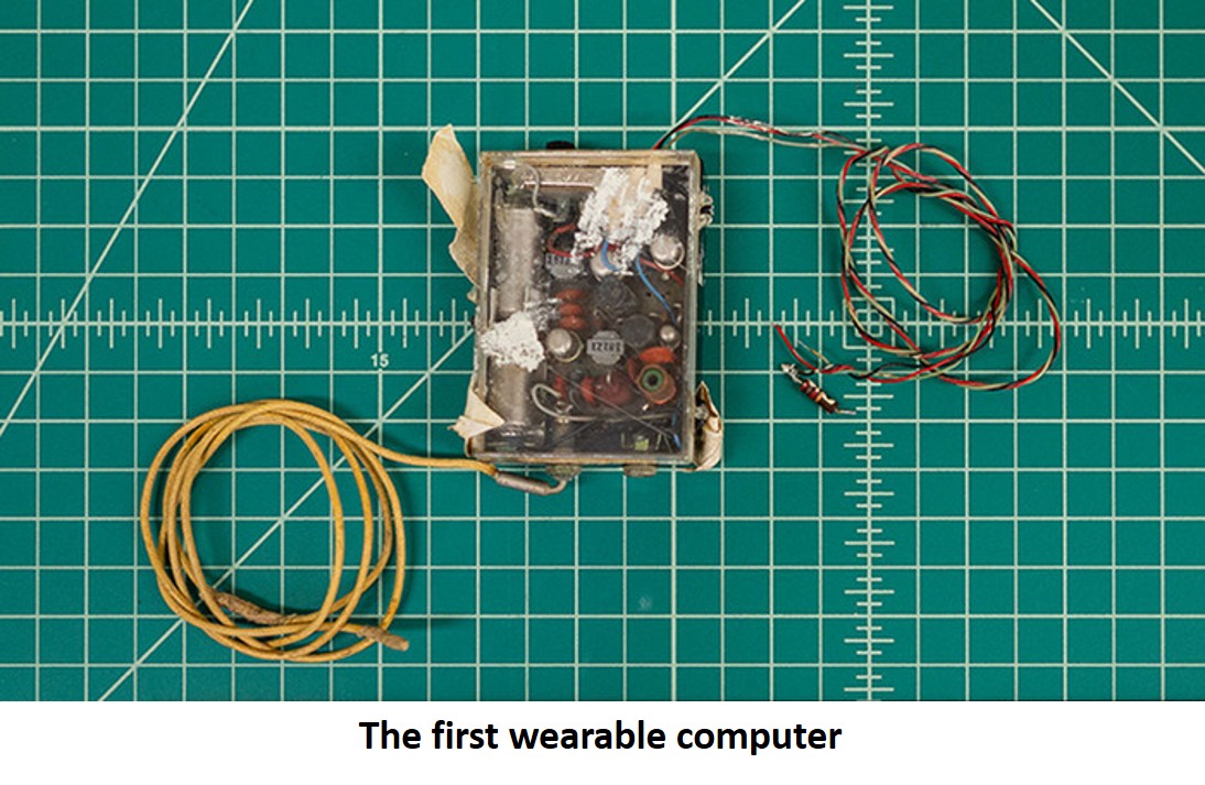
Image credits¶

• Forcing Function: John Kelly, Optimizing Investment Sizing with the Kelly Criterion
• Quanta Magazine: Claude Shannon, How Claude Shannon Invented the Future
• Life Magazine: Edward O. Thorp, The Professor Who Breaks the Bank, March 27 1964, pg 80
• UCI Libraries: First Wearable Computer, A Spin of the Wheel

Code and Software¶

Kelly.py - Kelly Criterion functions, plotReturnRatio.py and KellyMC.py

• Python: Python is an interpreted, high-level and general-purpose programming language.
• Tesseract OCR: Tesseract is an optical character recognition engine for various operating systems. It is free software, released under the Apache License.

See all software used on Wild Peaches →

References and further reading¶

• How Claude Shannon Invented the Future, Daved Tse, Quanta Magazine 22 Dec 2020.
• A Mathematical Theory of Communication, Claude Shannon, The Bell System Technical Journal, Jul 1948.
• A New Interpretation of Information Rate. J. L. Kelly, The Bell System Technical Journal, Jul 1956.
• Fortune's Formula: The Untold Story of the Scientific Betting System That Beat the Casinos and Wall Street. William Poundstone, Hill and Wang, 2005.
• Edward O. Thorp. Personal website.
• “He Was The First Man To Realize That The Electronic Computer Was Capable Of Analyzing All The Millions Of Possibilities”. Darren D’Addario, Afflictor, 2 May 2016.
• The Mathematics of Gambling. Edward O. Thorp,
• The Kelly Criterion and the Stock Market. Louis M. Rotando and Edward O. Thorp, American Mathematical Monthly, Dec 1992.
• The Invention of the First Wearable Computer. Edward O. Thorp

📬 Subscribe and stay in the loop. · Email · GitHub · Forum · Facebook

© 2020 – 2025 Jan De Wilde & John Peach