Fun with Physics

Home

keywords: physics modeling, Algodoo simulation, symbolic regression, HeuristicLab, physics education

Modern physics simulation tools and artificial intelligence are revolutionizing how we can understand and discover physical laws. This article will show you how to use these tools to explore physics concepts, test hypotheses, and even potentially discover new relationships – all without an advanced degree in theoretical physics.

The challenge many citizen scientists face is that traditional physics education requires years of mathematical training before you can start doing interesting experiments. But what if we could reverse this approach? What if we could use simulation tools to observe physical phenomena, collect data, and let artificial intelligence help us uncover the underlying mathematical relationships?

We'll explore how to:

• Use physics simulation software to run experiments
• Collect meaningful data from virtual experiments
• Apply symbolic regression to discover mathematical patterns
• Validate and understand the physics behind our findings

Through this process, you'll learn how modern tools are making physics more accessible to curious minds everywhere. Whether you're a hobbyist physicist, a student, or just someone fascinated by how the universe works, these techniques will help you explore physics concepts hands-on.

The Most Famous Equation¶

Probably the best-known equation is Albert Einstein's relationship between energy and matter,

It's only got three letters, and the most complicated part is $c^2$. Plot the equation and you'll see that it's just a straight line:

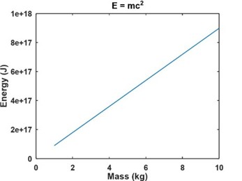
Other than realizing that energy is related to mass through the speed of light squared, you really phoned that one in, didn't ya Al?

Usually, scientists don't just think up the correct equation out of thin air. They collect data, test hypotheses, and fit equations to the data.

Physics Experiments in Algodoo¶

We need to have some data before making any hypotheses, and instead of building a miniature copy of the Cern Super Collider in the back yard, we'll use Algodoo. Algodoo simulates basic physical properties, is easy to set up and learn, there are user-contributed examples and an active community.

A simple example of Algodoo's capabilities is this inclined ramp with a ball. Hold the shift key down while drawing a polygon to get a ramp with straight edges, then add a circle. When you click the green arrow at the bottom of the screen the simulation starts and the ball rolls down. Reset the simulation by clicking the reset arrow just to the left of the start arrow.

On the right end of the control panel you'll see three buttons. These buttons control gravity, atmospheric drag, and the last turns on the background grid. A dark-gray background indicates that the feature is turned on, so in this case, both gravity and drag are active.

I thought that a good first experiment would be to collect data for a falling ball, first without drag and then with atmospheric drag turned on. I created a circle (ball), dragged it up to $48m$, and checked the physical properties by right-clicking the ball, and then clicking "Information":

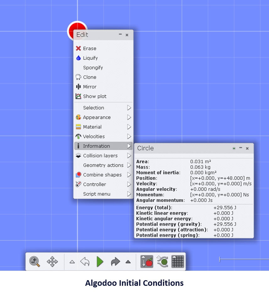
Notice that the drag has been turned off, but the grid is visible. Close the information window, and click on "Show plot" and run the simulation until the ball reaches the ground. It will bounce a few times, but you can stop it anytime after the first bounce.

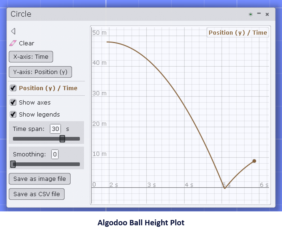
Click on the "Save as CSV file" button to save the data. Now we have some data, and it should be easy to see how well it fits the equation of an object falling under the influence of gravity only,

where $y(t)$ is the height at time $t$, $y_0=48m$ is the initial height, $v_y=0m/s$ is the initial velocity and $g=9.80665m/s^2$ is the standard acceleration due to gravity. Here's a plot generated in Octave of the data collected by Algodoo and the fitted positions:

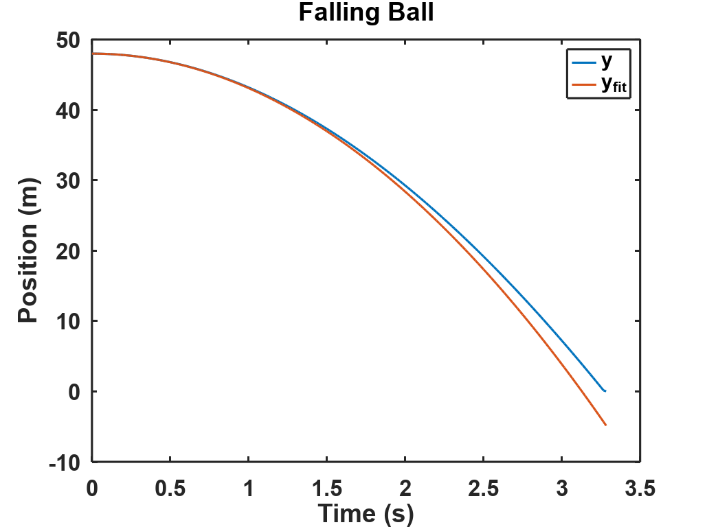
Something's wrong! Drag is turned off, so that's not it. Does Algodoo use a different gravitational acceleration constant? In the upper right corner of Algodoo, you'll see a small box with three icons. The lowest one looks like a magnifying glass, and if you click on that, a dialog box will appear showing Forces, Velocities, and Momentums:

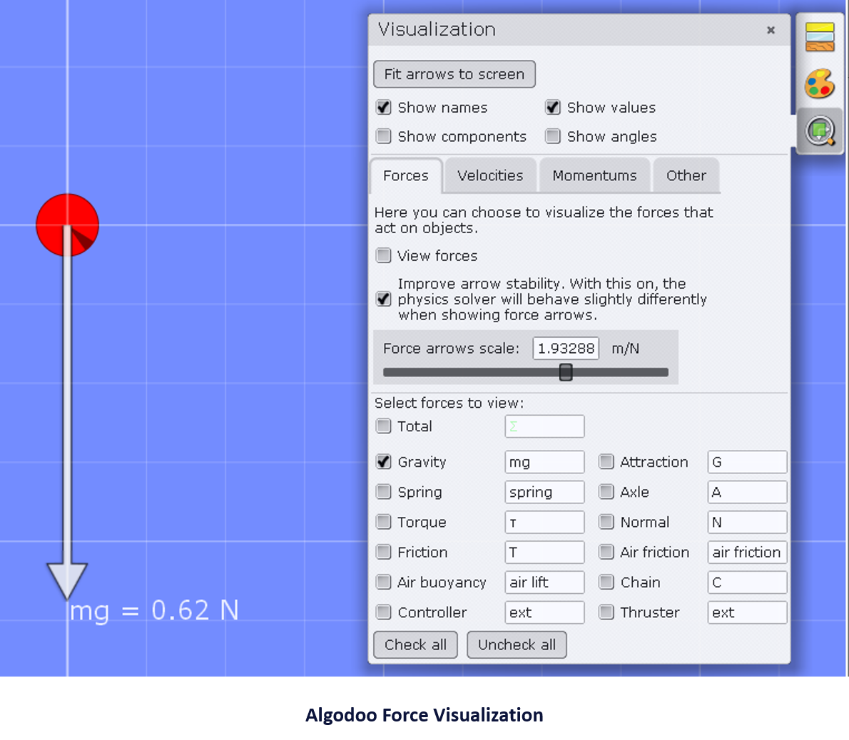
Since force = mass $\times$ acceleration ($F=ma$), we see that $mg=0.62N$ and the mass is $0.063kg$ so acceleration is

It's different, but not enough to correct the error, and it could be that it's due to round off error in the displayed force. In fact,

so rounding to two decimal places gives $mg=0.62N$ as shown. Octave has a function called polyfit that fits a polynomial to data, giving the coefficients to our falling object function,

>> c0 = polyfit(t,y,2)
c0 =
 
   -4.2439   -0.9725   48.2796

This says that the best fit is $y_0=48.2796m$, $v_y=-0.9725\frac{m}{s}$ and the gravitational acceleration is

That's soooo wrong! What is Algodoo doing? What is the actual equation being used to model the falling ball? To answer that we need to understand symbolic regression.

Symbolic Regression¶

Symbolic regression is a method that finds the best fitting function to a dataset. Defining best is difficult, though, because we need to trade off simplicity for accuracy. Of all the functions that come close to fitting the data, should we choose the one with the fewest terms or the one that most closely approximates the $y$ values? Before we get to that, we need to understand how symbolic regression works.

Computers store functions as expression trees where operators act on constants or variables, with the highest precedence operations taking place at the leaves of the tree and the lowest precedence taking place at the top. That sounds like gibberish, so let's take a look at the gravity function as an expression tree.

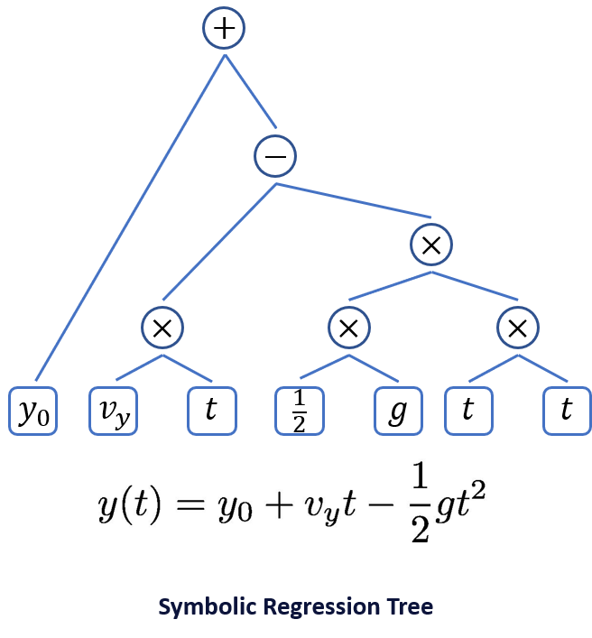
In the bottom right is $t\times t$ giving $t^2$, and next to that is the constant $\frac{1}{2}$ multiplied by the gravitational constant $g$. To the left, $v_y$ and $t$ are multiplied together to get the middle term. The acceleration term is subtracted from the velocity term using the minus operator, and finally, the initial position $y_0$ is added to complete the equation.

The way symbolic regression works is that the program generates hundreds of random expression trees like this and then combines them using a genetic algorithm. In a genetic algorithm, the population of expressions is paired off, the expression trees of each "parent" tree are snipped at some random point, and the snipped branches are swapped with the other parent to create two new offspring expressions. You might think of the expression as the DNA of an equation. Sheldon would say that the equations are having coitus.

The genetic algorithm chooses another equation to "mate" with the one shown above. It snips the "DNA" and swaps segments between the two expression trees.

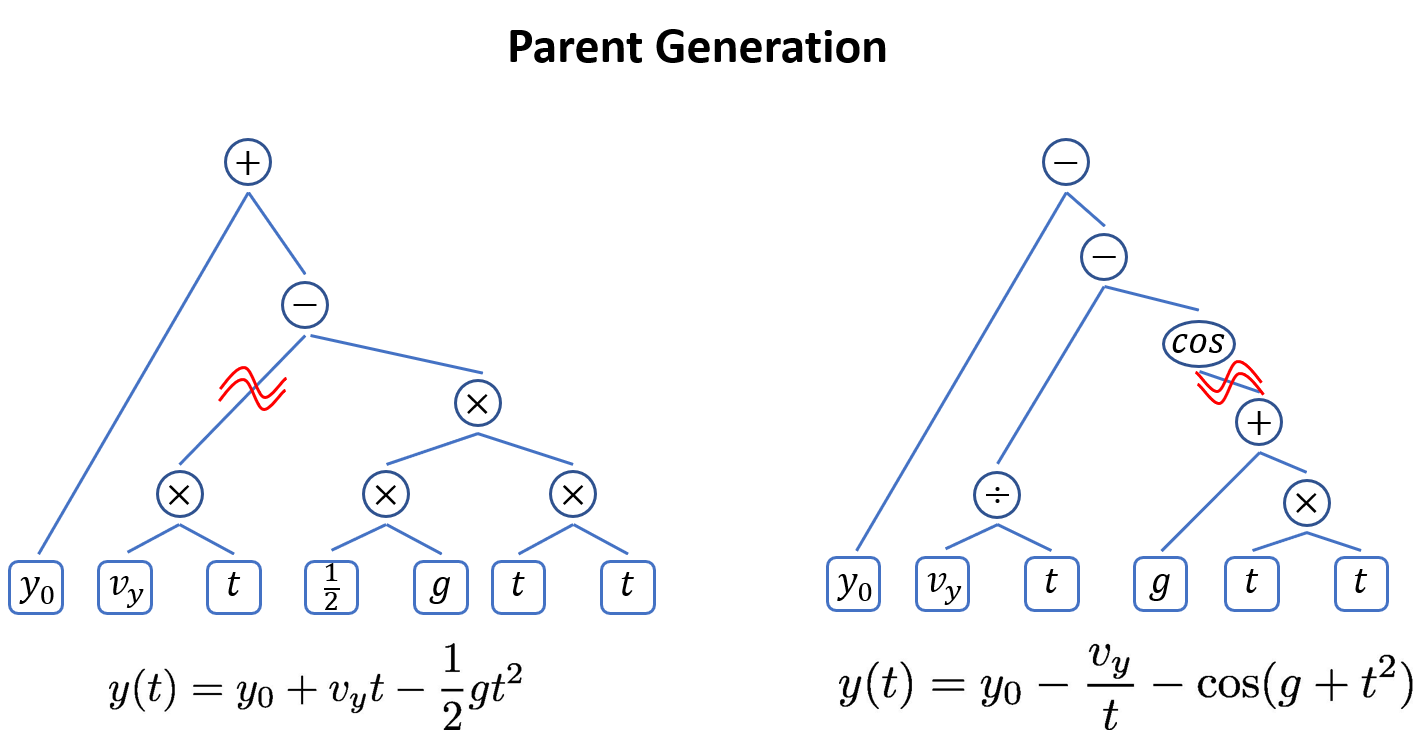
After swapping, the two new offspring equations are:

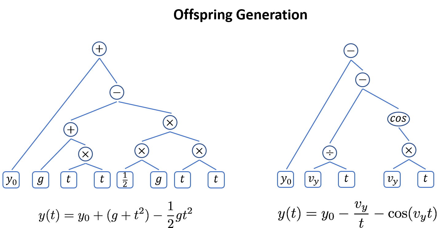
The two new equations are evaluated at each $t_i$ and compared to the data $y_i$ to see how well they fit. The algorithm might start with 1000 equations and generate another 1000 using this method. Each of the 2000 equations is evaluated at all times, and the top 1000 are kept for the next iteration. Amazingly, after a few hundred generations a good solution will often emerge.

Just as in nature, it's useful to have random mutations. Every once in a while, a constant gets changed, or an operator is swapped out for some other randomly selected operator. Usually, this results in a poorer fit, and the offspring is discarded, but sometimes you get an improvement that's worth keeping.

Writing a program to convert equations into tree expressions, and then handling all of the mechanics of the genetic algorithm is a lot of work. Fortunately, there are several open-source versions available. Dominic Searson wrote GPTips, which runs under Matlab. GPTips requires some coding to set up the model, but it works very well and you can select the model that gives good performance with minimal complexity.

TuringBot isn't open-source, but there is a free version, and AI Feynman 2.0 had been released recently which runs under Python. I've used GPTips, but not TuringBot or AI Feynman 2.0, although both look promising. But for now we'll use ...

HeuristicLab¶

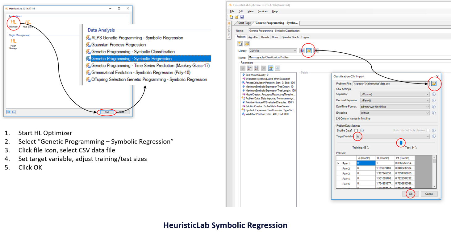
HeuristicLab has been in development at the Heuristic and Evolutionary Algorithms Laboratory (HEAL) for almost two decades and provides many genetic and machine learning algorithms in an easy-to-use GUI. From the About HeuristicLab page, "In HeuristicLab algorithms are represented as operator graphs and changing or rearranging operators can be done by drag-and-drop without actually writing code." Tutorials are available on the Documentation page, and you should spend some time watching the short video describing Symbolic Regression with HeuristicLab which walks through an example problem.

Open the data files generated by Algodoo and find the last row before the ball bounces. Delete all of the data below the bounce and save the file. Start HeuristicLab, select and start the Optimizer, and double click "Genetic Programming – Symbolic Regression". When the new tab opens click the file icon and select the data file. Change the target variable to "Position". For now, leave the Training/Test slider at 66%/34%.

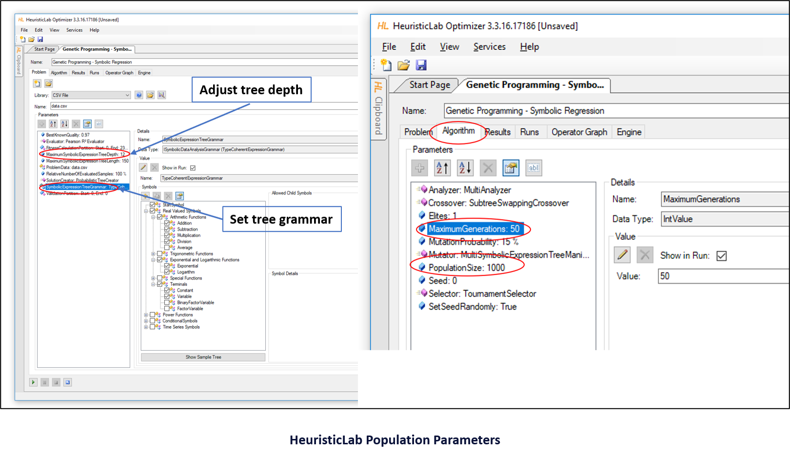
The default tree depth is 12, but this usually makes the fitted expression overly complicated. Try setting it to 6 to see if you can get a good fit. You can also change the tree grammar, that is, the operators available to the algorithm. Under the "Algorithm" tab, change the maximum number of generations and the population size, if you like.

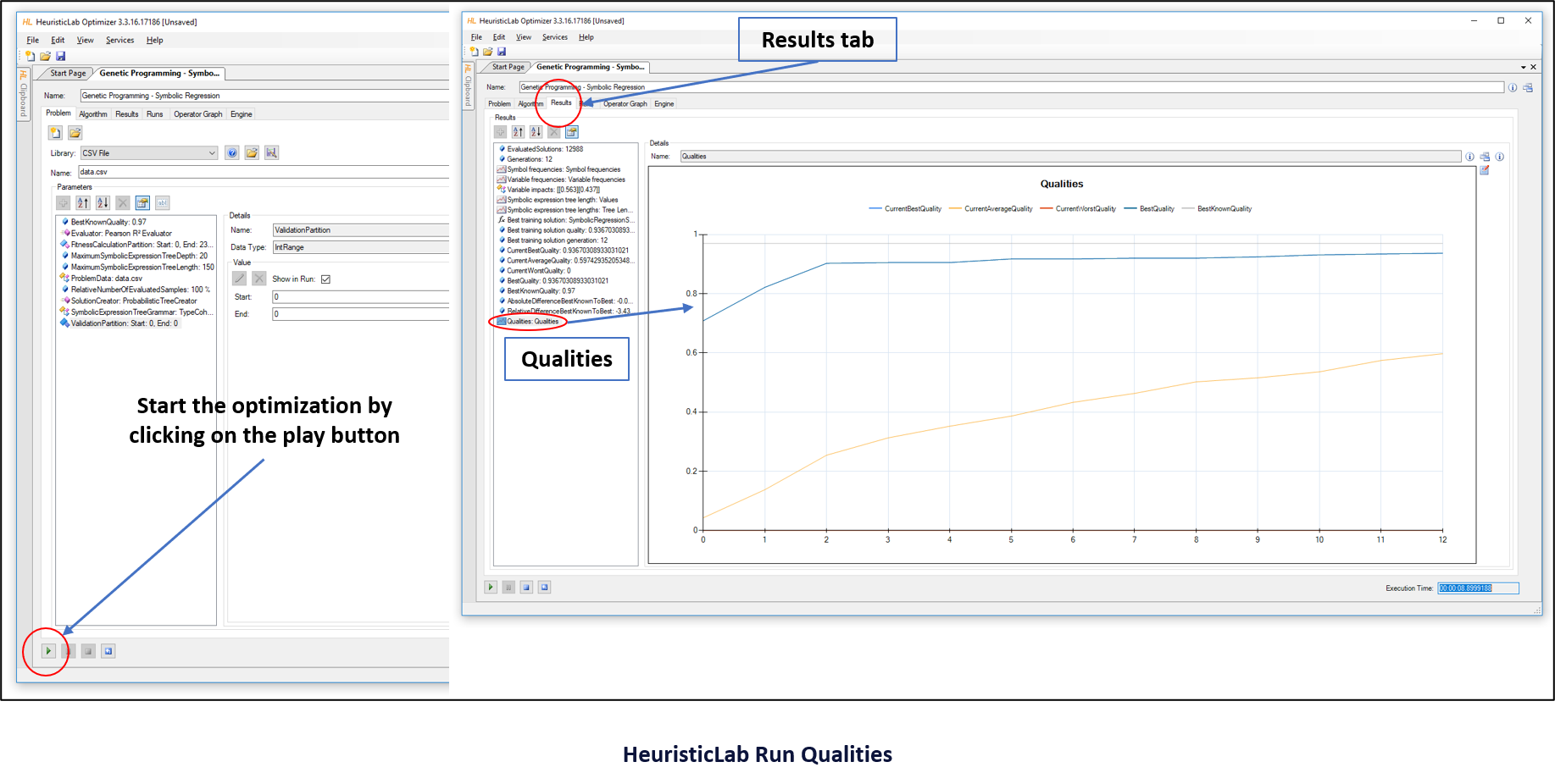
To start the symbolic regression, click on the green "Run" arrow in the bottom left corner. Switch to the "Results" tab, and select "Qualities" to watch the algorithm at work.

When the run has finished, click "Best Training Solution: SymbolicRegression" in the "Results" tab, and then double click "Model: Symbolic Regression Model".

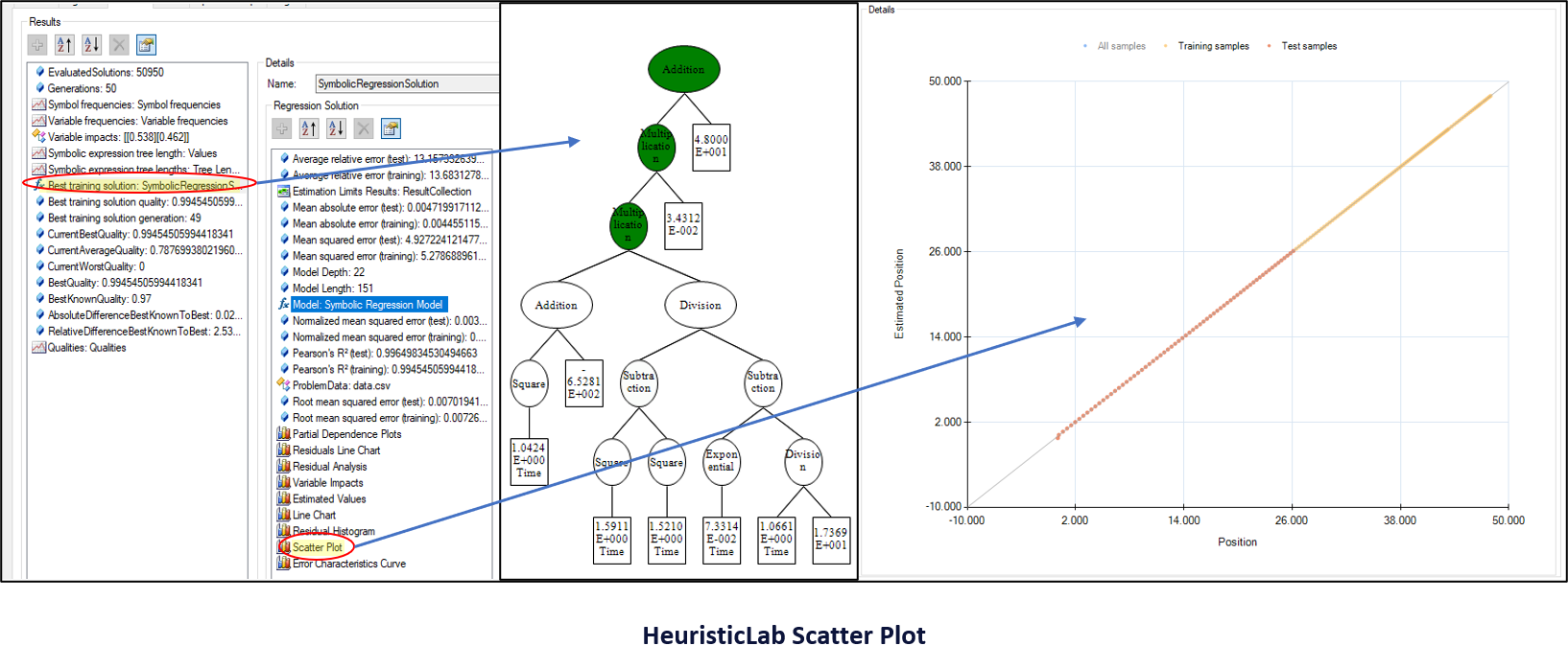
Click on "Test Samples" in the scatter plot to show the fit to both training and test data. You can simplify the model and optimize the parameters at this point. Watch the scatter plot as you make changes. If the scatter plot begins to deviate from the true values, you can undo simplifications.

HeuristicLab found this equation to best fit the data (right-click on the format icon for options):

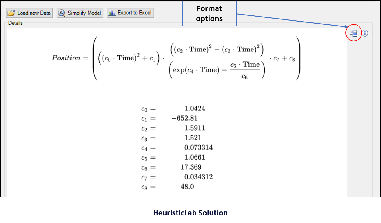
It's a very good fit, $R^2=0.99997458780501536$ on the test data, and probably would have been even better except that one test data point seems to be off the fit line. On the other hand, it's a very complex model for something that should have been much simpler. Reducing the tree depth would help, and since the population equations are chosen randomly, new runs produce different equations.

Final Thoughts¶

It seems unlikely that the physics model in Algodoo uses the equation that HeuristicLab found, but the data from Algodoo doesn't fit the gravity equation either. Maybe there's a gravity parameter setting somewhere in Algodoo that I missed, and I never got around to including atmospheric drag. The experiment could be re-run using a different physics engine such as ReactPhysics3D, SimPhy, Project Chrono, FisicaLab, or Bullet Physics.

Of course, the real fun with any symbolic regression engine would be to discover something new. You would need to find an unsolved problem, run the data through until you got a good fit, and then re-run multiple times to see if a simpler equation emerges. It's still up to you to figure out why the equation explains the phenomenon. Why are energy and matter related through the speed of light squared? Figuring that out makes for great science.

Code and Software¶

• Algodoo: Algodoo is a unique 2D-simulation physics software from Algoryx Simulation AB.
• Octave: GNU Octave is a high-level language, primarily intended for numerical computations.
• GPTips: a free Explainable-AI machine learning platform and interactive modelling environment for Matlab.
• TuringBot: TuringBot is a desktop software that uses Symbolic Regression to find mathematical formulas from data values.
• AI Feynman: an improved method for symbolic regression that seeks to fit data to formulas that are Pareto-optimal.
• HeuristicLab: HeuristicLab is a framework for heuristic and evolutionary algorithms, developed by the HEAL group.
• ReactPhysics3D: a C++ physics engine library that can be used in 3D simulations and games.
• SimPhy: SimPhy is a simulation software in Physics and Geometry, designed to visualize concepts such as free body diagrams.
• ProjectChrono: a physics-based modeling and simulation infrastructure written in C++.
• Bullet Physics: an open-source physics simulation library; also integrated in certain frameworks such as Kubric.

See all software used on Wild Peaches →

References and further reading¶

• The Big Bang Theory, Pilot episode 24 Sep 2007*. Chuck Lorre & Bill Prady, CBS.
• Nutty professor or one cool dude?*. M. Alex Johnson, NBC News, 15 Apr 2005
• Algoryx Simulation AB*. Developer of Algodoo.
• Heuristic and Evolutionary Algorithm Laboratory (HEAL)*. Research lab at University of Applied Sciences Upper Austria.

📬 Subscribe and stay in the loop. · Email · GitHub · Forum · Facebook

© 2020 – 2025 Jan De Wilde & John Peach