Julia Sets in Julia

Home

keywords: Julia sets, Julia language, complex numbers, iterated functions, fractals

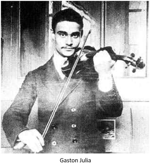
Gaston Julia¶

Gaston Julia was born on the 3rd of February, 1893 in Sidi bel Abbès, Algeria to Delorès Delavent and Joseph Julia, a mechanic. Gaston became interested in music and mathematics at an early age, and excelled in both, settling on the violin as his favorite instrument.

In 1901, the family moved to Oran on the coast of Algeria where he enrolled in the Lycée, eventually graduating with distinction in the baccalaureate examinations of science, modern languages, philosophy, and mathematics. He left Algeria for Paris and received a scholarship to the École Normale Supériore in 1911. In 1914 Germany declared war on France and Julia was called up for service with the 57th Infantry Regiment at Libourne.

Deployed to the Western Front, the following is a report of the action, and Julia's injury that cost him his nose.

January 25, 1915, showed complete contempt for danger. Under an extremely violent bombardment, he succeeded despite his youth (22 years) to give a real example to his men. Struck by a bullet in the middle of his face causing a terrible injury, he could no longer speak but wrote on a ticket that he would not be evacuated. He only went to the ambulance when the attack had been driven back. It was the first time this officer had come under fire.

For the remainder of his life, Julia wore a leather strap to cover the missing nose.

Julia married Marianne Chausson in 1918. She was the nurse who attended to him after his injury, and the daughter of composer Ernest Chausson. He had completed his Ph.D. in mathematics the year before, under Émile Picard, Henri Lebesgue, and Pierre Humbert.

At age 25, he published a 199-page manuscript, Mémoire sur l'iteration des fonctions rationelles, (Memoir on the iteration of rational functions) which brought him instant fame in mathematical circles and earned him the Grand Prix des Sciences Mathématiques of the French Academy of Sciences.

An iterated function is applied repeatedly to the previous solution, and a rational function is one like

where $P(x)$ and $Q(x)$ are polynomial functions. $Q(x)$ can't be zero, but it can be $1$, meaning that $f(x)=P(x)$.

Function Iterations¶

Iterating a function is pretty simple. Suppose

If you start with $x=0$, then $f(0)=1$. Now put $1$ into the function to get $f(1)=2$. This goes on forever, $1,2,3,\dots$ A more interesting function is

In other words, if $x$ is even, divide it by $2$, but if it's odd, multiply by $3$ and add $1$. Any number that's a power of $2$ immediately collapses down to $1$, for example, $x_0=8\Rightarrow f(8)=4\Rightarrow f(4)=2\Rightarrow f(2)=1$. Then you get stuck in the loop $4,2,1,4,2,1,\dots$ If you start with $3$ you get the sequence $\{3,10,5,16,8,4,2,1\}$.

Can you find a starting number that doesn't wind up at $1$? Nobody knows for sure, but it's thought that every sequence eventually winds down to $1$. This is known as the Collatz conjecture, named for mathematician Lothar Collatz who first proposed the conjecture in 1937. It's also called the Hailstone Problem because of the way the number sequence jumps up and down.

Curses, FOILed Again!¶

Remember the FOIL method from high school algebra? If you want to expand $(x+2)(x-3)$ using the FOIL method, you multiply the First two terms, $x\times x=x^2$, then the Outer terms, $x\times -3=-3x$, the Inner ones, $2\times x=2x$, and finally the Last two, $2\times -3=-6$ to get

Snidely Whiplash often said, "Curses, foiled again!" on the Rocky and Bullwinkle show, but he may not have been referring to algebra. Here's a picture of Rocky, Bullwinkle, and Captain Peachfuzz. Because reasons.

What's the square root of negative one $(\sqrt{-1})$? For a long time, mathematicians thought there was no solution to this problem because when you multiply two positive numbers together you get a positive number, and when you multiply two negative numbers together you also get a positive number, so there can't be an $x$ such that $x\times x=x^2=-1$. But, in the 17th century, René Descartes named the solution to $\sqrt{-1}$ as $i$, an imaginary, fictitious, and useless number.

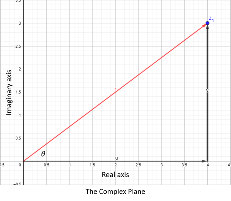
Since then, we've found plenty of uses for these otherwise useless numbers. Combine them with real numbers, the kind we're used to, and you get complex numbers like $4+3i$ which is $4$ parts real and $3$ parts imaginary. You can plot complex numbers as points, using the $x-$axis for the real part, and the $y-$axis for the imaginary part. Here's a plot of $z_1=4+3i$:

Suppose you wanted to multiply $z_1$ by another complex number $z_2=2+5i$. Just use the FOIL method but with the complex numbers,

Remember that $i^2=-1$, so multiplying the two imaginary parts together gives the negative of the product, ignoring the $i$'s. It might make more sense to do the first and last together to get the new real part, and then the inner and outer parts for the new imaginary. You could call it the FLIO method.

In the plot, the real part of $z_1$ is $4$, which is drawn as the vector $u$, and the imaginary part is $3$, drawn as the vector $v$. These two vectors form the adjacent and opposite sides of a right triangle with angle $\theta$. Using the Pythagorean Theorem, we can calculate the length of the hypotenuse, $r=\sqrt{4^2+3^2}=\sqrt{25}=5$. The sides $u$ and $v$ can be written in terms of $r$ and $\theta$ as

A Most Beautiful Equation¶

Leonard Euler (see our previous post, "Seven Bridges for Seven Truckers") discovered an amazing property of complex numbers,

where $e$ is the base of the natural logarithm. The proof is pretty simple. Define $f(\theta )$ as

The reason for choosing this particular function is that we will show that $f(\theta )=1$ for every $\theta$, meaning that the numerator and denominator are the same everywhere. Using the product rule of differentiation,

Since the derivative of $f(\theta )=0$ for every $\theta$, then $f(\theta )$ is a constant. The derivative of a function gives the slope of the function at every point, so a derivative of zero means the function has zero slope, in other words, it's a straight line parallel to the $x-$axis at some constant distance from the axis.

We can calculate the value of this constant at any $\theta$, and the easiest one is $\theta =0$, where $f(\theta )=1$ since $e^{-i\cdot 0}=1$, $\cos 0=1$, and $\sin 0=0$. In other words, $f(\theta )=1$ for every $\theta$, which completes the proof.

The angle $\theta$ is measured from the $x-$axis, so $\theta =0$ is along the positive real number line, $\theta =\frac{\pi }{2}$ is the positive imaginary axis, $\theta =\pi$ represents negative real numbers and $\theta =\frac{3\pi }{2}$ points along the negative imaginary axis.

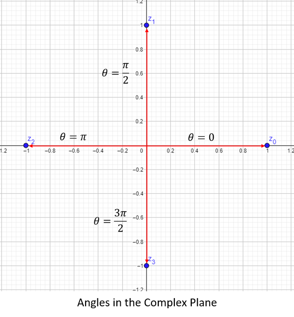
Looking at $z_2$, we see that when $\theta =\pi$, $e^{i\theta }=e^{i\pi }=-1$, which gives the most beautiful equation,

Physicist Richard Feynman said that this is "the most remarkable formula in mathematics" because it contains $e$, the base of natural logarithms, the imaginary number $i$, $\pi$, the constant relating the radius of a circle to its circumference and area, $1$ the first natural number, and $0$ the center of the mathematical universe.

Iterations on a Complex Number¶

Julia wondered what would happen if he iterated a function like $f(z)=z^2+c$ where both $z$ and $c$ could be complex. If $z=0$ and $c=1-i$, then the first few iterations become

If you start with a smaller $c$, say $c=-0.79+0.15i$, the values of $z$ jump around, but they stay relatively small. Another way to look at the iterations is to plot several steps of the iterations at different starting points $z_0$ and additive constant $c$.

Since the first iterate squares the initial value of $z_0$ and adds $c$, then $z_0=1$ and $z_0=-1$ will meet at $c+1$ after the first step. The same thing happens for $z_0=\pm i$.

In this plot, $z_0=(0.1+e^{i\theta })/2$ for $\theta =30,120,210,300$ degrees, and $c=-0.1+0.1i$.

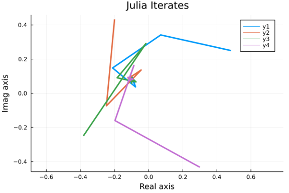
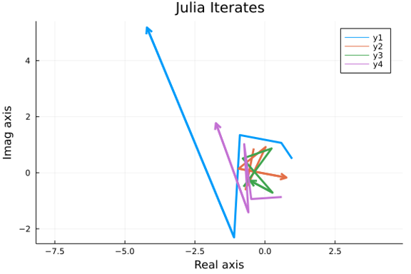
Adding $0.1$ shifts the starting points a little bit to prevent overlapping trajectories, and dividing by $2$ is equivalent to setting $r=\frac{1}{2}$ in the $u$ and $v$ vectors except for the slight shift of the starting point. If you set $z_0=0.1+e^{i\theta }$, eventually all of the trajectories escape towards infinity.

What is it that keeps some points from getting away, while others escape? The norm of a vector is the length of the vector and as we saw above, the length is easily calculated using the Pythagorean theorem. A shorthand notation for the norm is a pair of vertical lines around the vector or complex number,

After a single iteration, $z$ becomes $z^2+c$, and the length or norm is $|z^2+c|$. One way to check if the iterates are tending towards infinity is to calculate the length of each iterate. In the case $\theta =30°=0.52\text{ radians}$ (without dividing by $2$), the norm of the iterates is

Using the same starting point, and now dividing by $2$, the iterates are

Not only do the iterates remain small, but they get closer to $0.128$ (after rounding).

What happens if you write $z=r{e}^{i\theta }$ and want to find $z^2$? This is very easy because

How long is the new vector $z^2$? The $e^{2i\theta }$ part measures the angle so it doesn't contribute to the length, which means that the length of $z^2$ is simply $r^2$.

If we choose $c$ such that $|c|<1$, then $|z^2+c|$ will be greater than $1$ if $|z^2|>2$. If $r>1$ then $r^2$ will grow at each step. If you think of $z^2$ and $c$ as vectors, then the smallest value for $r$ is when $z^2$ and $c$ point in opposite directions.

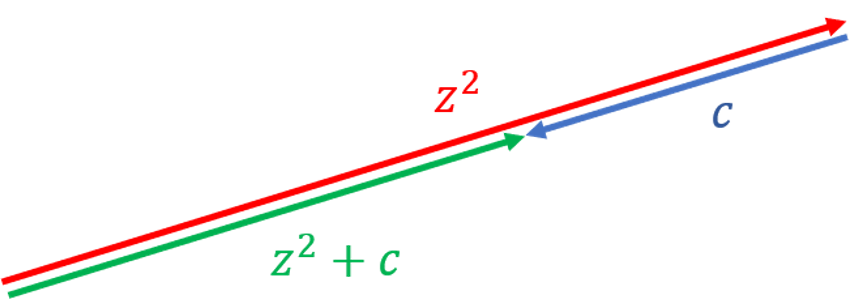
In most cases, $z^2$ and $c$ won't point in opposite directions, so $r$ will be even larger and the trajectory will escape faster, but we can check to see if $z^2>2$ and stop iterating when we get to that value.

Vectors are added together by connecting the point of $u$ to the tail of $v$ to get $z=u+v$. Subtracting $v$ from $u$ turns the direction of $v$ around.

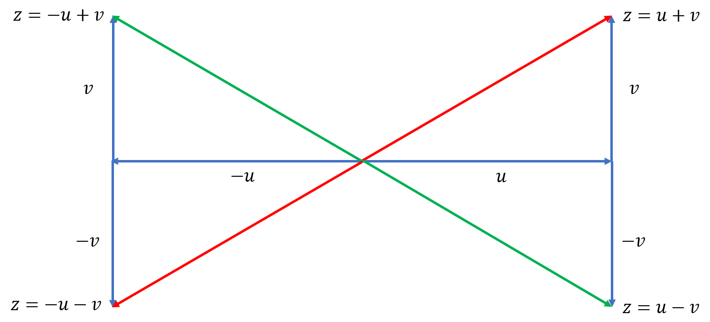
Using the FOIL method, we can calculate $z^2$ for combinations of positive and negative vectors $u$ and $v$.

In the picture above, you can see that the red $z$ vectors have the same $z^2$, as do the green vectors. After a single iteration, the new value of $z=u+v$ is the same as the new value of $z=-u-v$, just as the green vectors coincide. If $u+v$ results in an escaping trajectory, then so does $-u-v$.

Julia Sets¶

Gaston Julia wanted to find the boundary between the points that escaped and those that didn't. The boundary is now called the Julia Set. The $z$ points are taken from all points in the complex plane, and the set changes depending on the initial choice of the parameter $c$.

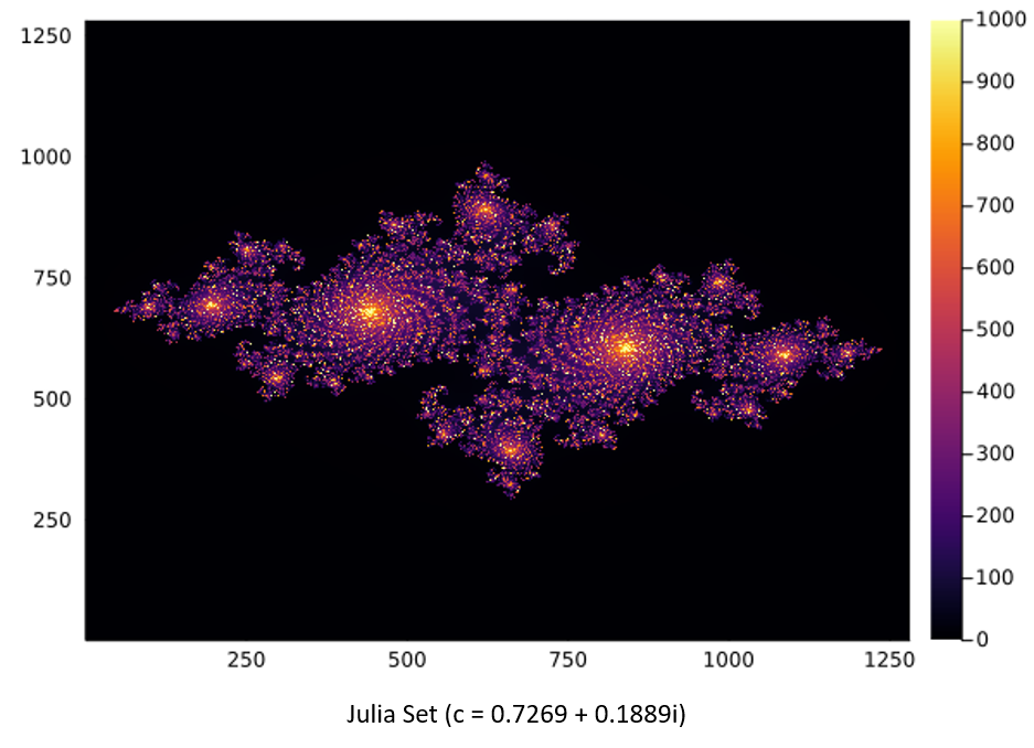
In this image, $c=-0.7269+0.1889i$, and the complex numbers range over $[-1.6,1.6]\times [-1.6,1.6]i$. The image is composed of 1281 points in each dimension, and for each point $z$, the number of iterations needed to exceed $|z|>2$ is stored in a matrix. The black regions are where $|z|$ starts greater than $2$, and the colored points are counts. On the right side, the color bar indicates the number of iterations, up to 1000, before the norm of $z$ becomes large.

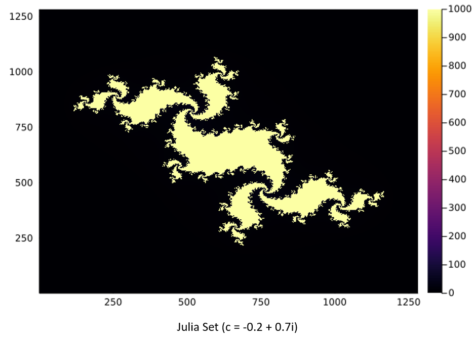
Another example shows that for $c=-0.20509091+0.71591i$, the points either are clearly in the set or outside. At the top of this post is a plot of the Julia set for values of $c$ from $c=-0.29609091+0.62491i$ to $c=-0.20509091+0.71591i$, taken from Benjamin Badger's Julia Sets page.

The code (on Github) to generate these images is very straightforward. An iterCounts array is initialized to zero, and for each $z$, the value of $|z_n|=|z_{n-1}^2+c|$ is computed. The iteration is repeated until either $|z_n|>2$ or the number of iterations reaches 1000. The array iterCounts is displayed as a heatmap to make the image.

The code is written in the Julia language because Julia is easy to learn and extremely fast. In fact, Julia is so fast that I didn't bother to take advantage of symmetry.

In the figure above, there are 1.6 million points and each point requires one multiplication and one addition to get $z_n=z_{n-1}^2+c$, and two more multiplications and an addition followed by a square root to get the norm of $z$. Even if only a quarter of the points got to the limit of 1000 iterations, somewhere near one billion calculations were required. In Julia, the whole process completed in just a little over 10 seconds even with inefficient code.

function plotJulia(c,xRng = [-1.6,1.6], yRng = [-1.6, 1.6])
    # Array of iteration counts
    nx = 1281
    ny = 1281
    iterCounts = zeros(nx,ny)
    # Locations
    xLocs = range(minimum(xRng),stop = maximum(xRng),length = nx)
    yLocs = range(minimum(yRng),stop = maximum(yRng),length = ny)
    # Loop over x,y locations iterating until maxIter reached, or |z|² > 4
    maxIters = 1000
    for j = 1:nx
        for k = 1:ny
            z = xLocs[j] + yLocs[k]im
            while iterCounts[j,k] < maxIters && norm(z) < 2
                z = z^2 + c
                iterCounts[j,k] += 1
            end
        end
    end
 
    # Display Julia set as a heatmap
    display(heatmap(iterCounts'))
 
    # Return array of iteratations
    return iterCounts
 
end

Exploring the Infinite Beauty of Julia Sets¶

The journey through the world of Julia sets reveals the intricate beauty and complexity that arise from simple mathematical iterations. By exploring the boundary between points that escape to infinity and those that remain bounded, we uncover stunning fractal patterns that captivate mathematicians and artists alike.

If you'd like to go deeper, consider experimenting with different values of the complex parameter $c$ to generate your own unique Julia sets. The Julia programming language, with its speed and ease of use, provides an excellent platform for these explorations. You could also look at the relationship between Julia sets and the Mandelbrot set, another fascinating fractal that serves as a map of all possible Julia sets.

You might also consider investigating the applications of complex dynamics in fields such as computer graphics, chaos theory, and even natural phenomena. The interplay between mathematics and art in fractals offers endless possibilities for creative expression and scientific inquiry.

Gaston Julia never saw the images that we can now quickly produce in the Julia language, but he was able to work out many of the details and provide great insight into the structure of Julia sets.

Image credits¶

• Hero: Julia sets. Benjamin Badger, Form and Formula, 2023.
• Gaston Julia: Gaston Maurice Julia. Edmund Robertson and John O'Connor, MacTutor, School of Mathematics and Statistics at the University of St Andrews.
• Curses Foiled Again: The Darkest Minds. Jessica Darke, Amused in the Dark, 2018.
• Rocky and Bullwinkle: Rocky & Bullwinkle’s triumphant return. Eric Norcross, Renegade Cinema, Nov 6, 2013.

Code and Software¶

JuliaSetPlots.jl - Plots trajectories and filled Julia sets: plotIterates, plotJulia

• Julia - The Julia Project as a whole is about bringing usable, scalable technical computing to a greater audience: allowing scientists and researchers to use computation more rapidly and effectively; letting businesses do harder and more interesting analyses more easily and cheaply.
• VSCode and VSCodium - Visual Studio Code is a lightweight but powerful source code editor which runs on your desktop and is available for Windows, macOS and Linux. It comes with built-in support for JavaScript, TypeScript and Node.js and has a rich ecosystem of extensions for other languages and runtimes (such as C++, C#, Java, Python, PHP, Go, .NET). VSCodium is a community-driven, freely-licensed binary distribution of Microsoft’s editor VS Code.
• Pluto.jl - Pluto is an environment to work with the Julia programming language. Easy to use like Python, fast like C.

References¶

• Julia, G. (1918). "Mémoire sur l’itération des fonctions rationnelles". Journal de Mathématiques Pures et Appliquées.
• MacTutor History of Mathematics Archive (n.d.). Gaston Julia. University of St Andrews.
• Devaney, R. L. (1989). "Computers, Fractals and Dynamics: Computer Experiments in Mathematics". Addison-Wesley.
• Devaney, R. L. (2012). "Chaos, Fractals and Dynamics: Computer Experiments in Mathematics". YouTube Video.
• Sutherland, S. (n.d.). "An Introduction to Julia and Fatou Sets". Stony Brook University.
• Avalos-Bock, S. (2009). "Fractal Geometry: The Mandelbrot and Julia Sets". University of Chicago.
• Kuennen, E. (n.d.). "Chaotic Dynamics and Fractals.". University of Wisconsin Oshkosh.
• Sims, K. (n.d.). "Understanding Julia and Mandelbrot Sets". Karl Sims' Research Page.
• Badger, B. (n.d.). Julia Sets. Personal Blog.
• Plots.jl Documentation (n.d.). Julia Language Plots.jl and Plot Attributes. JuliaLang.
• Wikipedia (n.d.). Julia Set. Wikipedia.
• JuliaLang (n.d.). The Julia Programming Language. JuliaLang.
• Julia Bloggers (n.d.). Timing in Julia. JuliaBloggers.
• Wikipedia (n.d.). Collatz Conjecture. Wikipedia.

📬 Subscribe and stay in the loop. · Email · GitHub · Forum · Facebook

© 2020 – 2025 Jan De Wilde & John Peach