
keywords: curve fitting, Weierstrass approximation, Hubbert peak theory, Seneca cliff, polynomial approximation
"How did you go bankrupt?” Bill asked.
"Two ways,” Mike said. “Gradually, then suddenly."
—Ernest Hemingway, The Sun Also Rises
The Weierstrass Approximation Theorem
In 1885, Karl Weierstrass
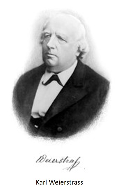
proved that any continuous function can be approximated as closely as you like with a polynomial. Written in mathematical terms, the theorem he proved is
Theorem: Suppose f : [ 0 , 1 ] ⇒ R f:[0,1] \Rightarrow \mathbb{R} f:[0,1]⇒R is continuous. For any ϵ > 0 \epsilon > 0 ϵ>0, there exists a polynomial p p p such that
sup x ∈ [ 0 , 1 ] ∣ f ( x ) − p ( x ) ∣ ≤ ϵ . {\text{sup} \atop x \in [0,1]} |f(x)-p(x)| \leq \epsilon. x∈[0,1]sup∣f(x)−p(x)∣≤ϵ.What does all this mean? Let's start with f : [ 0 , 1 ] ⇒ R f: [0,1] \Rightarrow \mathbb{R} f:[0,1]⇒R. This says that the function f f f takes any value of x x x between 0 0 0 and 1 1 1 and returns a real-valued number, y = f ( x ) y = f(x) y=f(x) and y y y can be anything. A function is continuous if it exists at every x x x and you can trace the curve without lifting your pencil.
The part about "For any ϵ > 0 \epsilon > 0 ϵ>0" is a trick mathematicians use a lot, and it means if you think of some very small positive number, we can always find another even smaller, but still positive number. The way we use this very, very tiny ϵ \epsilon ϵ is to take the absolute value of the difference between f ( x ) f(x) f(x) and p ( x ) p(x) p(x) at every x x x and make sure it's less than ϵ \epsilon ϵ.
The sup x ∈ [ 0 , 1 ] \text{sup} \atop x \in [0,1] x∈[0,1]sup is not "'Sup, dude?", but it's short for supremum and it means that for all possible polynomials p p p approximating f f f, we want to choose the one where the maximum absolute value difference between f ( x ) f(x) f(x) and p ( x ) p(x) p(x) for any x x x in the interval [ 0 , 1 ] [0,1] [0,1] is the minimum. In other words, we want to choose the p p p which minimizes the biggest error.
You might be wondering why the x − x- x−values are constrained to be between 0 0 0 and 1 1 1, and the answer is, it doesn't matter. You can shrink, stretch and shift x x x to fit any interval. Suppose your function is defined over the interval [ a , b ] [a,b] [a,b]. Then, for every x x x, make
x ′ = x − a b − a x' = \frac{x-a}{b-a} x′=b−ax−aso when x = a x=a x=a, x ′ = 0 x' = 0 x′=0 and when x = b x=b x=b, x ′ = 1 x'=1 x′=1. Then modify your function to
g ( x ) = ( b − a ) f ( x ) + a g(x) = (b-a)f(x)+a g(x)=(b−a)f(x)+aand you get the same y y y values as f f f, but over the interval [ 0 , 1 ] [0,1] [0,1].
A theorem isn't a theorem until it's been proved. Weierstrass proved his theorem, but in 1912, Sergei Bernstein
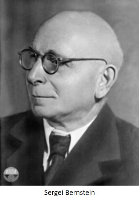
used Bernstein basis polynomials to construct approximation functions. In "Yacht Design with Mathematics" we used Bernstein polynomials as the basis for Bezier functions. For any n ≥ 0 n \geq 0 n≥0, the n + 1 n+1 n+1 Bernstein basis polynomials are defined as
B k , n = ( n k ) x k ( 1 − x ) n − k , k = 0 , 1 , 2 , … , n B_{k,n}={n \choose k} x^k (1-x)^{n-k}, \; k=0,1,2,\ldots,n Bk,n=(kn)xk(1−x)n−k,k=0,1,2,…,nwith x x x in the interval [ 0 , 1 ] [0,1] [0,1]. The Binomial Theorem shows how to expand the polynomial in x x x and y y y to the n t h n^{th} nth power,
( x + y ) n = ∑ k = 0 n ( n k ) x k − n y k . (x+y)^n = \sum_{k=0}^n {n \choose k} x^{k-n}y^k. (x+y)n=k=0∑n(kn)xk−nyk.Substitute y = 1 − x y = 1-x y=1−x, add up all k k k Bernstein polynomials and you get,
∑ k = 1 n B k , n ( x ) = ( x + ( 1 − x ) ) n = 1 n = 1 \sum_{k=1}^n B_{k,n}(x) = (x + (1-x))^n = 1^n = 1 k=1∑nBk,n(x)=(x+(1−x))n=1n=1for any x x x. Bernstein then defined a new function which included a continuous function f f f on the interval [ 0 , 1 ] [0,1] [0,1] to be
B n ( f ) ( x ) = ∑ k = 0 n f ( k n ) B k , n ( x ) = ∑ k = 0 n f ( k n ) ( n k ) x k ( 1 − x ) n − k . B_n(f)(x) = \sum_{k=0}^n f\left( \frac{k}{n} \right) B_{k,n}(x) = \sum_{k=0}^n f\left( \frac{k}{n} \right) {n \choose k} x^k (1-x)^{n-k}. Bn(f)(x)=k=0∑nf(nk)Bk,n(x)=k=0∑nf(nk)(kn)xk(1−x)n−k.Michael Bertrand gives the complete version of Bernstein's proof in his article, "Bernstein Proves the Weierstrass Approximation Theorem", and I'll provide another version at the end.
In 1938, Marshall Stone

extended Weierstrass' Theorem which is now known as the Stone-Weierstrass Theorem.
Some Applications
What can you do with a polynomial approximation to a function? With a good polynomial fit, you can use the polynomial to estimate the derivative or the integral of f f f, and this is what is done with software packages like Chebfun for Matlab, ApproxFun in Julia, or Python libraries such as pychebfun, ChebPy, or PaCAL. Polynomials are easy to differentiate and integrate, which is often not true for arbitrary functions, so having a good approximation is quite useful. These software tools can approximate continuous functions to machine precision, and computing with polynomials is fast.
With an approximate derivative or integral you can solve differential equations, and this has led to applications in neural networks as described in "Universal Invariant and Equivariant Graph Neural Networks". For insight into how Chebfun works, see "Chebfun: A New Kind of Numerical Computing" by Platte and Trefethen. The Chebfun website has many examples,
- Rational approximation of the Fermi-Dirac function describing the distribution of energy states for systems of particles.
- A drowning man and Snell's Law is derived from Fermat's principle giving the refraction of light through different media.
- Exponential, logistic, and Gompertz growth. "The Boonie Conundrum" used the Gompertz function to model the spread of a rumor.
- Procrustes shape analysis. We talked about the Greek myth of Procrustes in "Designing the Model".
- Modeling infectious disease outbreaks. In "How Deep Is That Pool?" we showed how to calculate the optimal pool size for COVID-19 testing.
- Smoothies: nowhere analytic functions. Weierstrass found functions that are continuous everywhere, but not differentiable anywhere.
You'll find plenty of nerdy-cool projects to try out. The only negative aspect of Chebfun is it requires the commercial software Matlab, but you may find an open-source version you prefer in Chebfun-related projects.
Polynomials aren't the only way to approximate functions. Fourier approximation and wavelets are other methods, and Nick Trefethen has written the book, "Approximation Theory and Approximation Practice" (partially available online). See the Publications page for other references.
Something you should never do is fit a function f f f with a high degree polynomial p p p and then extrapolate p p p beyond the limits of f f f. You only get a good fit over the interval [ a , b ] [a,b] [a,b] where you defined f f f.
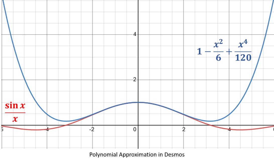
Here, the function
f ( x ) = sin ( x ) x f(x) = \frac{\sin(x)}{x} f(x)=xsin(x)may be approximated by the polynomial
p ( x ) = 1 − x 2 6 + x 4 120 . p(x)=1 - \frac{x^2}{6} + \frac{x^4}{120}. p(x)=1−6x2+120x4.Between − π 2 -\frac{\pi}{2} −2π and π 2 \frac{\pi}{2} 2π the fit is pretty good, but outside the interval, the fit is much worse.
A Naive Approach to Approximations
Suppose you knew nothing about approximation theory and decided to try fitting one function (or data) with the sum of a simpler function?
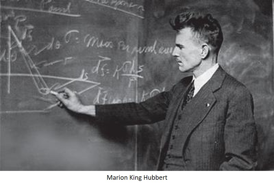
Marion King Hubbert was a geologist, mathematician, and physicist who worked for Shell Oil, the USGS, and taught at Columbia, Stanford, and UC Berkeley. In 1956, he looked at oil production data and proposed a model for the amount of oil extracted from a field,
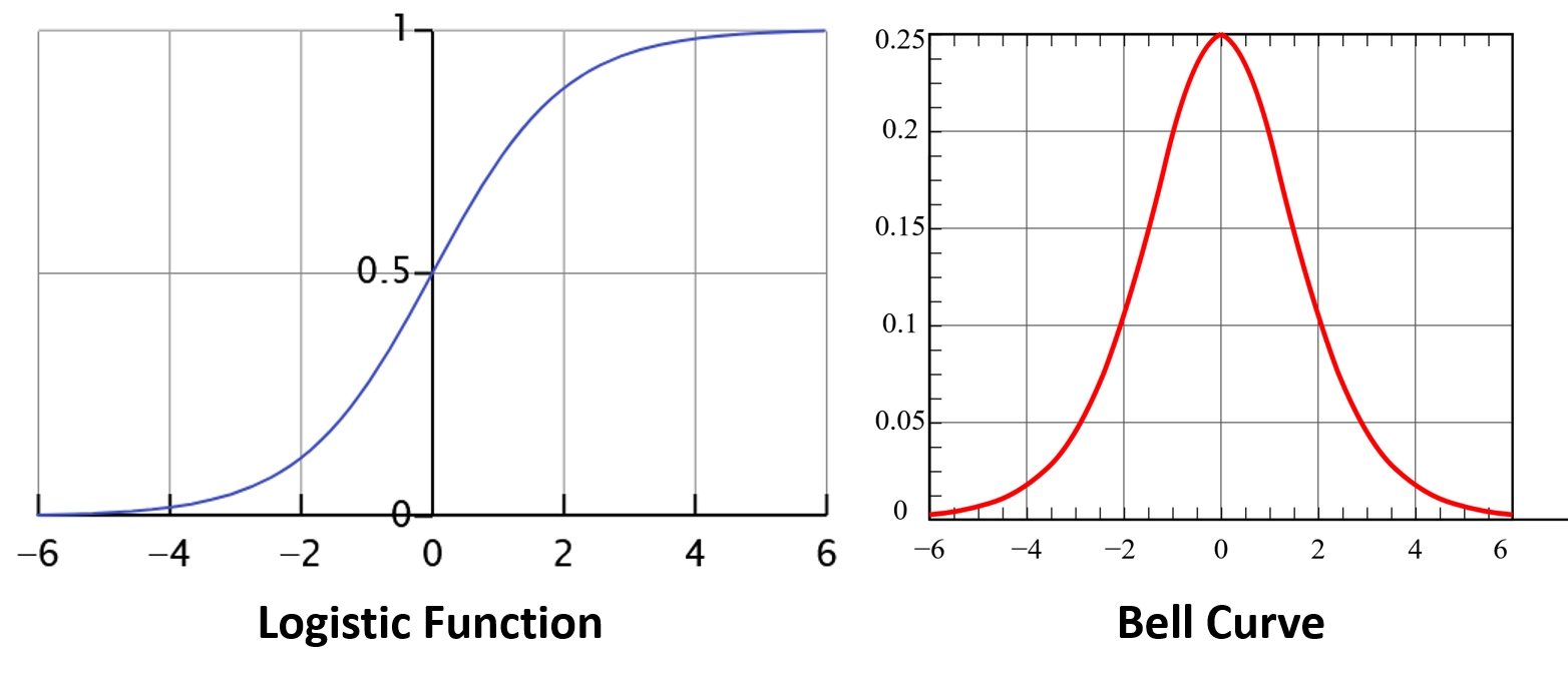
Q ( t ) = Q max 1 + a e − b t Q(t) = \frac{Q_{\text{max}}}{1+ae^{-bt}} Q(t)=1+ae−btQmaxwhere Q max Q_{\text{max}} Qmax is the total quantity of oil to eventually be produced from the field, Q ( t ) Q(t) Q(t) is the cumulative production up to time t t t, and constants a a a and b b b are parameters defined by local geology. This is the logistic function first described by Pierre Francois Verhulst to model population growth. The derivative of the logistic function produces a bell-shaped curve (or Gaussian function), which for Hubbert was the instantaneous rate of oil flow from the field.
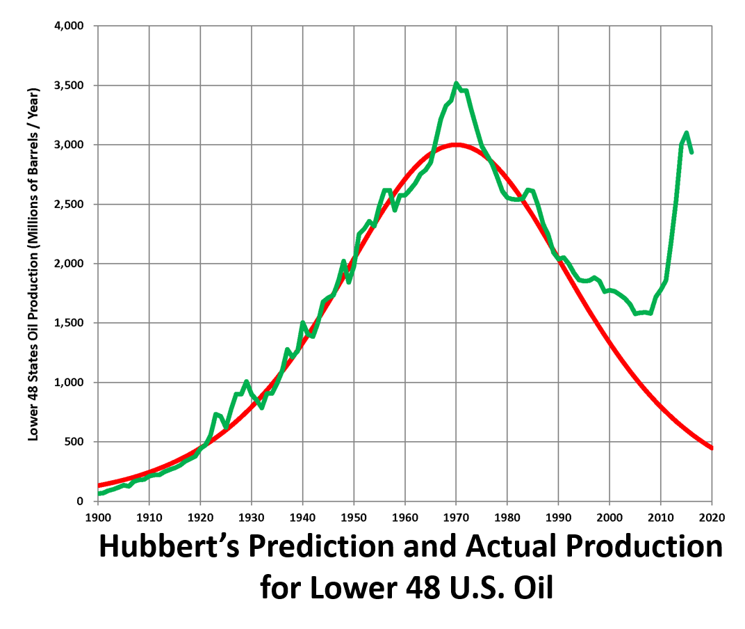
Hubbert used the logistic function because initially with only a few wells production would be low, but as more came on line production should increase. Eventually, though, depletion would slow the rate of production. Hubbert thought his model could be extended to all U.S. oil production and predicted the peak of production would occur in 1970 for the lower 48 states.
In 1976 Hubbert predicted the world peak in production might happen as soon as 1995. A 2007 study by the UK Energy Resource Center found no geological reason to expect cumulative oil production should follow a logistic curve. They reported on field data suggesting peaks tended to happen at about 25% of the total production Q max Q_\text{max} Qmax.
On the other hand, Ugo Bardi says decline is faster than growth and likes to quote Seneca,
"It would be some consolation for the feebleness of our selves and our works if all things should perish as slowly as they come into being; but as it is, increases are of sluggish growth, but the way to ruin is rapid." Lucius Anneaus Seneca, Letters to Lucilius, n. 91

We can model individual fields using Gaussian functions,
g ( t ) = α e − ( t − μ ) 2 2 σ 2 g(t) = \alpha e^{-\frac{(t-\mu)^2}{2 \sigma^2}} g(t)=αe−2σ2(t−μ)2where α \alpha α represents the peak amount produced, μ \mu μ is the time of peak production and σ \sigma σ determines the width of the bell curve. The Ghawar field in Saudi Arabia produces tens of thousands of barrels per day ( α \alpha α), has been in operation since μ = 1948 \mu = 1948 μ=1948, and continues to this day so σ \sigma σ is large. More recently, U.S. shale wells have increased production (the green curve departing from Hubbert's prediction), but their peaks are much lower and production drops 90% from the peak after only three years.
Is it possible to generate Bardi's Seneca Cliff with a series of Gaussians? Using Julia, the Seneca Cliff can be modeled as
f(x) = 0 < x <= 1 ? x : 0which asks the question, Is x x x between 0 0 0 and 1 1 1? If it is, f ( x ) = x f(x) = x f(x)=x, otherwise it's zero.
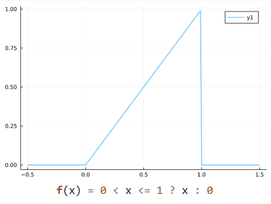
If oil production mimicked this f ( x ) f(x) f(x), the rate would increase linearly until suddenly every oil well in the world stopped producing on the same day. This is about as likely as Zaphod Beeblebrox's Infinite Improbability Drive, but we're just trying to build a simple mind-sized problem. "See, all my procedures are mind-sized bites", explains seventh-grader Robert in Seymour Papert's Mindstorms.
First we need to create a vector of x − x- x−values,
x = Array(-0.5:0.01:1.5));and then the corresponding y − y- y−values using a list comprehension
y = [f(x_i) for x_i in x];Next, for each value of the parameters α , μ \alpha, \mu α,μ and σ \sigma σ we can define a function g g g and evaluate it over x x x,
g(x,α,μ,σ) = sum( α[i] * exp( - (x-μ[i])^2/(2*σ[i]^2) ) for i = 1:n)or
g ( x , α , μ , σ ) = ∑ i = 1 n α i exp ( − ( x − μ i ) 2 2 σ i 2 ) . g(x,\alpha,\mu,\sigma) = \sum_{i=1}^n \alpha_i \exp \left( - \frac{(x-\mu_i)^2}{2 \sigma_i^2} \right). g(x,α,μ,σ)=i=1∑nαiexp(−2σi2(x−μi)2).which gives an estimate for y y y using the sum of n n n Gaussians
y_fit = [g(x_i,α,μ,σ) for x_i in x]Using the LsqFit.jl package, we'll get the best parameters to fit f ( x ) f(x) f(x). LsqFit requires an initial estimate, so I chose
α i = 1 − 1 2 i μ i = 1 − 1 2 i σ i = 1 4 i \begin{aligned} \alpha_i &= 1 - \frac{1}{2^i} \\ \mu_i &= 1 - \frac{1}{2^i} \\ \sigma_i &= \frac{1}{4^i} \end{aligned} αiμiσi=1−2i1=1−2i1=4i1and then created an initial vector p 0 = [ α ; μ ; σ ] ; p_0 = [\alpha; \mu; \sigma]; p0=[α;μ;σ]; with n = 4 n=4 n=4. To get the fit, LsqFit uses the function curve_fit
fit = curve_fit(gaussSum, x, y, p₀, lower = lb, upper = ub)where gaussSum contains the definition for
g
g
g, extracts the parameters from
p
0
p_0
p0, and generates
y
_
fit
y\_\text{fit}
y_fit. The values of the parameters
α
,
μ
\alpha, \mu
α,μ and
σ
\sigma
σ are required to be between the lower bound lb and the upper bound ub which were set to zero and one for this example.
The result is a pretty good approximation
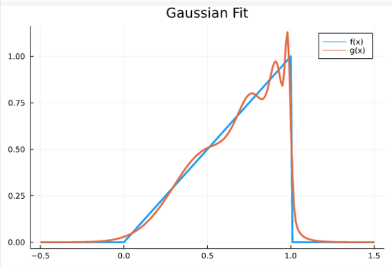
You can see the peaks of each Gaussian with centers μ = [ 0.52 , 0.80 , 0.93 , 0.99 ] \mu = [0.52, 0.80, 0.93, 0.99] μ=[0.52,0.80,0.93,0.99] and widths σ = [ 0.218 , 0.099 , 0.041 , 0.014 ] \sigma = [0.218, 0.099, 0.041, 0.014] σ=[0.218,0.099,0.041,0.014]. The optimal amplitudes are α = [ 0.51 , 0.57 , 0.63 , 0.69 ] \alpha = [0.51, 0.57, 0.63, 0.69] α=[0.51,0.57,0.63,0.69]. The function f f f has a discontinuity at x = 1 x=1 x=1, so we wouldn't be able to find a polynomial approximation. Smoothing over the discontinuity would help with the sum of Gaussians technique. This doesn't mean this model necessarily represents what's actually happening, but it shows that a sum of Gaussian-like production curves can still lead to a Seneca Cliff. The Julia code is on GitHub.
This is a good experimental start to finding a method for fitting Gaussians to functions. Is there a pattern to the values for α , μ \alpha, \mu α,μ and σ \sigma σ? Can you find a functional representation for the parameters that works for different n n n? What happens if you change f f f? Can you find a general rule giving the parameters for any f f f and any n n n? Test your hypotheses by changing f f f (line 17) and plotting the fit.
The Proof
Here's the proof of Weierstrass' theorem. It's actually pretty easy to follow if you take it in mind-size bites. It comes from Chris Tisdell, a mathematician at UNSW Sydney. The proof below was taken from his YouTube video and is based on the proof by Dunham Jackson.
Introduction to the Theorem:
- Statement: Any continuous function defined on a closed interval [ a , b ] [a,b] [a,b] can be uniformly approximated by a polynomial to any desired degree of accuracy.
- Importance: Establishes the foundation for polynomial approximation in analysis.
Key Concepts:
- Uniform Approximation: The concept that the maximum difference between the function and the approximating polynomial can be made arbitrarily small.
- Continuous Functions: Functions that are unbroken and have no gaps over the interval [ a , b ] . [a,b]. [a,b].
Constructing the Polynomial:
-
Bernstein Polynomials: Introduction of Bernstein polynomials as a constructive method to approximate continuous functions.
-
Definition: For a function f ( x ) f(x) f(x) on [ 0 , 1 ] [0,1] [0,1], the n n n-th Bernstein polynomial is given by:
B n ( f , x ) = ∑ k = 0 n f ( k n ) ( n k ) x k ( 1 − x ) n − k . B_n(f,x)= \sum_{k=0}^n f \left( \frac{k}{n} \right) \binom{n}{k} x^k(1−x){n−k}. Bn(f,x)=k=0∑nf(nk)(kn)xk(1−x)n−k.
Proof Outline:
- Step 1: Approximation on
[
0
,
1
]
[0, 1]
[0,1]:
- Show that B n ( f , x ) B_n(f, x) Bn(f,x) converges uniformly to f ( x ) f(x) f(x) on [ 0 , 1 ] [0,1] [0,1] n → ∞ n \to \infty n→∞.
- Use properties of binomial coefficients to demonstrate convergence for large n n n.
- Step 2: Extension to
[
a
,
b
]
[a, b]
[a,b]:
- Use a linear transformation to map the interval [ a , b ] [a,b] [a,b] to [ 0 , 1 ] [0,1] [0,1].
- Apply the approximation on [ 0 , 1 ] [0,1] [0,1] to the transformed function.
- Step 3: Uniform Convergence:
- Prove that the maximum deviation ∣ f ( x ) − B n ( f , x ) ∣ |f(x) - B_n(f, x)| ∣f(x)−Bn(f,x)∣ can be made less than any ϵ > 0 \epsilon > 0 ϵ>0 for sufficiently large n n n.
- Use the properties of continuous functions and compactness of the interval to ensure uniform convergence.
Theorem: Suppose f : [ a , b ] ⇒ R f: [a,b] \Rightarrow \mathbb{R} f:[a,b]⇒R is a continuous function. Then we can construct a sequence of polynomials P n P_n Pn such that for any ϵ > 0 \epsilon > 0 ϵ>0 there exists N = N ( ϵ ) N = N(\epsilon) N=N(ϵ) such that for all x ∈ [ a , b ] x \in [a,b] x∈[a,b] we have
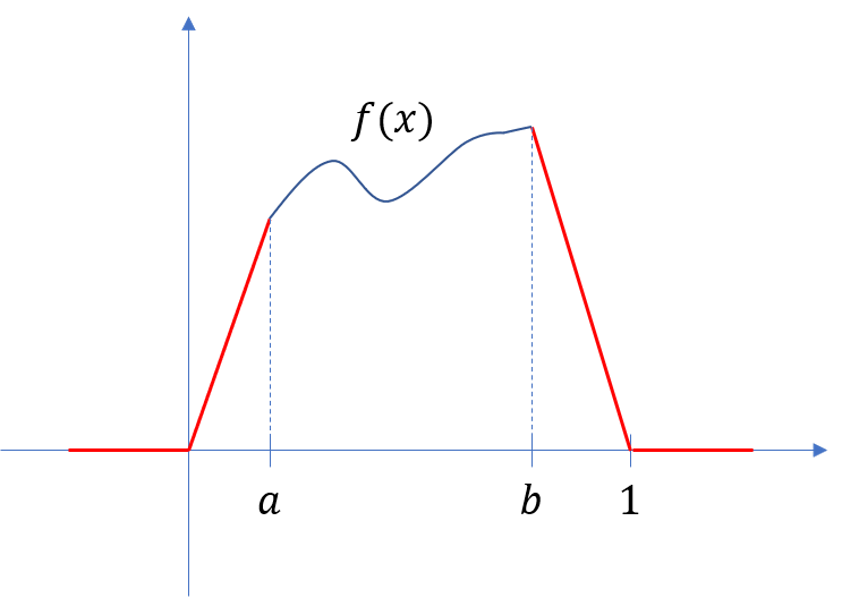
∣ P n ( x ) − f ( x ) ∣ < ϵ , for all n > N . |P_n(x) - f(x)| < \epsilon, \text{ for all } n > N. ∣Pn(x)−f(x)∣<ϵ, for all n>N.Proof: Assume 0 < a < b < 1 0 < a < b < 1 0<a<b<1. Extend f f f to the entire real line by defining
f ( x ) = { 0 , if x ≤ 0 x a f ( a ) , if 0 < x < a f ( x ) , if a ≤ x ≤ b 1 − x 1 − b f ( b ) , if b < x < 1 0 , if x ≥ 1 f(x) = \left\{ \begin{array}{ll} 0, & \text{if } x \leq 0 \\ \frac{x}{a}f(a), & \text{if } 0 < x < a \\ f(x), & \text{if } a \leq x \leq b \\ \frac{1-x}{1-b}f(b), & \text{if } b < x < 1 \\ 0, & \text{if } x \geq 1 \end{array} \right. f(x)=⎩⎨⎧0,axf(a),f(x),1−b1−xf(b),0,if x≤0if 0<x<aif a≤x≤bif b<x<1if x≥1This just adds pieces to f ( x ) f(x) f(x) so that it covers the entire real line by connecting ( 0 , 0 ) (0,0) (0,0) to ( a , f ( a ) ) (a,f(a)) (a,f(a)) and ( b , f ( b ) ) (b,f(b)) (b,f(b)) to ( 1 , 0 ) (1,0) (1,0), and then defining f ( x ) = 0 f(x) = 0 f(x)=0 for any point outside the interval [ 0 , 1 ] [0,1] [0,1], (and it's still continuous)
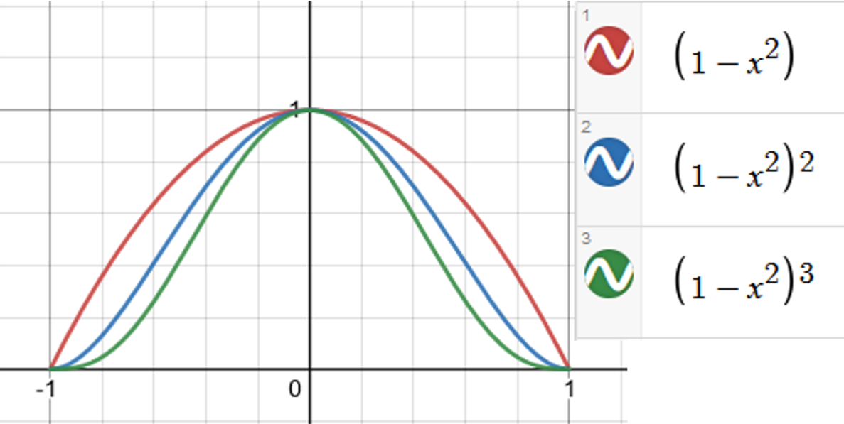
Now, create a sequence of constants (called a Landau integral),
J n : = ∫ − 1 1 ( 1 − u 2 ) n d u . J_n := \int_{-1}^1 (1-u^2)^n du. Jn:=∫−11(1−u2)ndu.Here are some examples of the Landau integral, and the numeric values over the interval [ − 1 , 1 ] [-1,1] [−1,1]. Integration gives the area below the curve and above the x − x- x−axis.
Next, define polynomials using these constants,
P n ( x ) : = 1 J n ∫ 0 1 f ( t ) ( 1 − ( t − x ) 2 ) n d t . P_n(x) := \frac{1}{J_n}\int_0^1 f(t) \left( 1 - (t-x)^2 \right)^n dt. Pn(x):=Jn1∫01f(t)(1−(t−x)2)ndt.The first three polynomials of the sequence are
P 1 ( x ) = 1 J 1 ∫ 0 1 f ( t ) ( 1 − ( t − x ) 2 ) d t P 2 ( x ) = 1 J 2 ∫ 0 1 f ( t ) ( 1 − ( t − x ) 2 ) 2 d t P 3 ( x ) = 1 J 3 ∫ 0 1 f ( t ) ( 1 − ( t − x ) 2 ) 3 d t . \begin{aligned} P_1(x) &= \frac{1}{J_1} \int_0^1 f(t) (1-(t-x)^2) dt \\ P_2(x) &= \frac{1}{J_2} \int_0^1 f(t) (1-(t-x)^2)^2 dt \\ P_3(x) &= \frac{1}{J_3} \int_0^1 f(t) (1-(t-x)^2)^3 dt. \end{aligned} P1(x)P2(x)P3(x)=J11∫01f(t)(1−(t−x)2)dt=J21∫01f(t)(1−(t−x)2)2dt=J31∫01f(t)(1−(t−x)2)3dt.The idea is when n n n gets to be big enough, P n ( x ) P_n(x) Pn(x) will very closely match f ( x ) f(x) f(x). Notice that the degree of P n ( x ) P_n(x) Pn(x) is at most 2 n 2n 2n.
Since f ( x ) = 0 f(x) = 0 f(x)=0 for every x x x outside of the interval [ 0 , 1 ] [0,1] [0,1] then
P n ( x ) = 1 J n ∫ 0 1 f ( t ) ( 1 − ( t − x ) 2 ) n d t = 1 J n ∫ − 1 + x 1 + x f ( t ) ( 1 − ( t − x ) 2 ) n d t = 1 J n ∫ − 1 1 f ( x + u ) ( 1 − u 2 ) n d u . \begin{aligned} P_n(x) &= \frac{1}{J_n}\int_0^1 f(t) \left( 1 - (t-x)^2 \right)^n dt \\ &= \frac{1}{J_n}\int_{-1+x}^{1+x} f(t) \left( 1 - (t-x)^2 \right)^n dt \\ &= \frac{1}{J_n}\int_{-1}^1 f(x+u) \left( 1 - u^2 \right)^n du. \\ \end{aligned} Pn(x)=Jn1∫01f(t)(1−(t−x)2)ndt=Jn1∫−1+x1+xf(t)(1−(t−x)2)ndt=Jn1∫−11f(x+u)(1−u2)ndu.Changing the limits of integration from 0 to 1 in the first line to − 1 + x -1+x −1+x to 1 + x 1+x 1+x in the second line doesn't really do anything for x ∈ [ 0 , 1 ] x \in [0,1] x∈[0,1] except it now runs over [ − 1 , 2 ] [-1,2] [−1,2] instead. In other words, let
g ( t ) = f ( t ) ( 1 − ( t − x ) 2 ) n g(t) = f(t) \left( 1 - (t-x)^2 \right)^n g(t)=f(t)(1−(t−x)2)nso
∫ 0 1 g ( t ) d t = ∫ − 1 + x 0 g ( t ) d t + ∫ 0 1 g ( t ) d t + ∫ 1 1 + x g ( t ) d t \int_0^1 g(t) dt = \int_{-1+x}^0 g(t)dt + \int_0^1 g(t)dt + \int_1^{1+x} g(t)dt ∫01g(t)dt=∫−1+x0g(t)dt+∫01g(t)dt+∫11+xg(t)dtwhere the first and third terms are zero since f ( x ) f(x) f(x) is zero on those intervals, leaving the middle term unchanged.
If we change variables, letting u = t − x u = t-x u=t−x so t = u + x t = u+x t=u+x, then d t = d u dt = du dt=du. The limits of the integral change from
t = − 1 + x ⇒ u + x = − 1 + x ⇒ u = − 1 t = 1 + x ⇒ u + x = 1 + x ⇒ u = 1. \begin{aligned} t &= -1 + x \Rightarrow u+x=-1+x \Rightarrow u = -1 \\ t &= 1+x \Rightarrow u+x=1+x \Rightarrow u = 1. \end{aligned} tt=−1+x⇒u+x=−1+x⇒u=−1=1+x⇒u+x=1+x⇒u=1.Now, look at the difference between this polynomial approximation P n ( x ) P_n(x) Pn(x) and the function we want to approximate f ( x ) f(x) f(x),
P n ( x ) − f ( x ) = 1 J n ∫ − 1 1 f ( x + u ) ( 1 − u 2 ) n d u − f ( x ) = 1 J n ∫ − 1 1 [ f ( x + u ) − f ( x ) ] ( 1 − u 2 ) n d u \begin{aligned} P_n(x) - f(x) &= \frac{1}{J_n}\int_{-1}^1 f(x+u) \left( 1 - u^2 \right)^n du - f(x) \\ &= \frac{1}{J_n}\int_{-1}^1 \left[ f(x+u) - f(x) \right] \left( 1 - u^2 \right)^n du \end{aligned} Pn(x)−f(x)=Jn1∫−11f(x+u)(1−u2)ndu−f(x)=Jn1∫−11[f(x+u)−f(x)](1−u2)nduwhere we use the Landau integral
J n = ∫ − 1 1 ( 1 − u 2 ) n d u 1 = 1 J n ∫ − 1 1 ( 1 − u 2 ) n d u f ( x ) = 1 J n ∫ − 1 1 f ( x ) ( 1 − u 2 ) n d u . \begin{aligned} J_n &= \int_{-1}^1 (1-u^2)^n du \\ 1 &= \frac{1}{J_n} \int_{-1}^1 (1-u^2)^n du \\ f(x) &= \frac{1}{J_n} \int_{-1}^1 f(x) (1-u^2)^n du. \\ \end{aligned} Jn1f(x)=∫−11(1−u2)ndu=Jn1∫−11(1−u2)ndu=Jn1∫−11f(x)(1−u2)ndu.Since f f f is continuous, then for any ϵ > 0 \epsilon > 0 ϵ>0 there is a δ \delta δ such that
∣ f ( x + u ) − f ( x ) ∣ < ϵ 2 , for all ∣ u ∣ < δ . | f(x+u) - f(x)| < \frac{\epsilon}{2}, \text{ for all } |u| < \delta. ∣f(x+u)−f(x)∣<2ϵ, for all ∣u∣<δ.If M M M is the maximum value of ∣ f ∣ |f| ∣f∣ then
∣ f ( x + u ) − f ( x ) ∣ ≤ 2 M , for all u |f(x+u) - f(x)| \leq 2M, \text{ for all } u ∣f(x+u)−f(x)∣≤2M, for all usince ∣ f ( x + u ) ∣ ≤ M |f(x+u)| \leq M ∣f(x+u)∣≤M and ∣ f ( x ) ∣ ≤ M |f(x)| \leq M ∣f(x)∣≤M, then
∣ f ( x + u ) − f ( x ) ∣ ≤ ∣ f ( x + u ) ∣ + ∣ f ( x ) ∣ ≤ M + M = 2 M . |f(x+u)-f(x)| \leq |f(x+u)| + |f(x)| \leq M + M = 2M. ∣f(x+u)−f(x)∣≤∣f(x+u)∣+∣f(x)∣≤M+M=2M.For any ∣ u ∣ > δ |u| > \delta ∣u∣>δ, then u 2 > δ 2 u^2 > \delta^2 u2>δ2, so
1 ≤ u 2 δ 2 1 \leq \frac{u^2}{\delta^2} 1≤δ2u2and therefore
∣ f ( x + u ) − f ( x ) ∣ ≤ 2 M u 2 δ 2 . |f(x+u)-f(x)| \leq \frac{2Mu^2}{\delta^2}. ∣f(x+u)−f(x)∣≤δ22Mu2.In either case, ∣ f ( x + u ) − f ( x ) ∣ |f(x+u)-f(x)| ∣f(x+u)−f(x)∣ must be less than the sum of these two bounds, so
∣ f ( x + u ) − f ( x ) ∣ ≤ ϵ 2 + 2 M u 2 δ 2 . |f(x+u)-f(x)| \leq \frac{\epsilon}{2} + \frac{2Mu^2}{\delta^2}. ∣f(x+u)−f(x)∣≤2ϵ+δ22Mu2.With these bounds, we can write
∣ P n ( x ) − f ( x ) ∣ = 1 J n ∫ − 1 1 [ f ( x + u ) − f ( x ) ] ( 1 − u 2 ) n d u ≤ 1 J n ∫ − 1 1 [ ϵ 2 + 2 M u 2 δ 2 ] ( 1 − u 2 ) n d u = 1 J n ∫ − 1 1 ϵ 2 ( 1 − u 2 ) n d u + 1 J n ∫ − 1 1 2 M u 2 δ 2 ( 1 − u 2 ) n d u = ϵ 2 1 J n ∫ − 1 1 ( 1 − u 2 ) n d u + 2 M δ 2 J n ∫ − 1 1 u 2 ( 1 − u 2 ) n d u = ϵ 2 + 2 M δ 2 J n ∫ − 1 1 u 2 ( 1 − u 2 ) n d u . \begin{aligned} |P_n(x) - f(x)| &= \frac{1}{J_n}\int_{-1}^1 \left[ f(x+u) - f(x) \right] (1 - u^2)^n du \\ &\leq \frac{1}{J_n}\int_{-1}^1 \left[ \frac{\epsilon}{2} + \frac{2Mu^2}{\delta^2} \right] (1 - u^2)^n du \\ &= \frac{1}{J_n}\int_{-1}^1 \frac{\epsilon}{2} (1 - u^2)^n du + \frac{1}{J_n}\int_{-1}^1 \frac{2Mu^2}{\delta^2} (1 - u^2)^n du \\ &= \frac{\epsilon}{2} \frac{1}{J_n}\int_{-1}^1 (1 - u^2)^n du + \frac{2M}{\delta^2 J_n}\int_{-1}^1 u^2 (1 - u^2)^n du \\ &= \frac{\epsilon}{2} + \frac{2M}{\delta^2 J_n}\int_{-1}^1 u^2 (1 - u^2)^n du. \\ \end{aligned} ∣Pn(x)−f(x)∣=Jn1∫−11[f(x+u)−f(x)](1−u2)ndu≤Jn1∫−11[2ϵ+δ22Mu2](1−u2)ndu=Jn1∫−112ϵ(1−u2)ndu+Jn1∫−11δ22Mu2(1−u2)ndu=2ϵJn1∫−11(1−u2)ndu+δ2Jn2M∫−11u2(1−u2)ndu=2ϵ+δ2Jn2M∫−11u2(1−u2)ndu.Let
I n = ∫ − 1 1 u 2 ( 1 − u 2 ) n d u I_n = \int_{-1}^1 u^2 (1 - u^2)^n du In=∫−11u2(1−u2)nduand then using integration by parts ( ∫ μ d ν = μ ν − ∫ ν d μ \int \mu d\nu = \mu \nu - \int \nu d \mu ∫μdν=μν−∫νdμ) and letting
μ = u ⇒ d μ = 1 d ν = u ( 1 − u 2 ) n ⇒ ν = ( 1 − u 2 ) n ( u 2 − 1 ) 2 ( n + 1 ) = − 1 2 ( n + 1 ) J n + 1 . \begin{aligned} \mu &= u \Rightarrow d \mu = 1 \\ d \nu &= u(1-u^2)^n \Rightarrow \nu = \frac{(1-u^2)^n(u^2-1)}{2(n+1)} = -\frac{1}{2(n+1)}J_{n+1}. \end{aligned} μdν=u⇒dμ=1=u(1−u2)n⇒ν=2(n+1)(1−u2)n(u2−1)=−2(n+1)1Jn+1.So this means the integral I n I_n In can be bounded by J n / 2 n J_n/2n Jn/2n,
I n = 0 + 1 2 ( n + 1 ) J n + 1 < J n 2 n . I_n = 0 + \frac{1}{2(n+1)}J_{n+1} < \frac{J_n}{2n}. In=0+2(n+1)1Jn+1<2nJn.In other words,
∣ P n ( x ) − f ( x ) ∣ ≤ ϵ 2 + 2 M δ 2 J n I n < ϵ 2 + 2 M δ 2 J n J n 2 n = ϵ 2 + 2 M 2 n δ 2 = ϵ 2 + ϵ 2 = ϵ \begin{aligned} |P_n(x) - f(x)| &\leq \frac{\epsilon}{2} + \frac{2M}{\delta^2 J_n}I_n \\ &< \frac{\epsilon}{2} + \frac{2M}{\delta^2 J_n}\frac{J_n}{2n} \\ &= \frac{\epsilon}{2} + \frac{2M}{2n \delta^2}\\ &= \frac{\epsilon}{2} + \frac{\epsilon}{2} = \epsilon \end{aligned} ∣Pn(x)−f(x)∣≤2ϵ+δ2Jn2MIn<2ϵ+δ2Jn2M2nJn=2ϵ+2nδ22M=2ϵ+2ϵ=ϵso long as n n n is sufficiently large such that
2 M 2 n δ 2 < ϵ 2 . ■ \frac{2M}{2n \delta^2} < \frac{\epsilon}{2}. \; \blacksquare 2nδ22M<2ϵ.■Image credits
- Hero: Oil EIR Raises Sticky Issues For Hermosa Beach. Dana Murray, Heal the Bay, Apr. 14, 2014.
- Karl Weierstrass: Wikimedia Commons.
- Sergei Bernstein: Wikipedia.
- Marshall Stone: Marshall Harvey Stone seated in a classroom, ca. 1974. University of Massachusetts Amherst. Special Collections and University Archives, University of Massachusetts Amherst Libraries.
- Marion King Hubbert: Wikipedia.
- Hubbert Prediction Lower 48: Wikimedia Commons.
- The Seneca Cliff: The Seneca Effect. Ugo Bardi, The Seneca Effect: why decline is faster than growth. Aug 28, 2011.
- Dunham Jackson: Wikimedia Commons.
Code for this article
fitGaussParams.jl - Estimates parameters required to fit sum of Gaussians to a function: fitParams, gaussSum, plotFit
- Desmos - is an advanced graphing calculator implemented as a web application and a mobile application. In addition to graphing both equations and inequalities, it also features lists, plots, regressions, interactive variables, graph restriction, simultaneous graphing, piece wise function graphing, polar function graphing, two types of graphing grids – among other computational features commonly found in a programmable calculator.
- Julia - The Julia Project as a whole is about bringing usable, scalable technical computing to a greater audience: allowing scientists and researchers to use computation more rapidly and effectively; letting businesses do harder and more interesting analyses more easily and cheaply.
- VSCode and VSCodium - Visual Studio Code is a lightweight but powerful source code editor which runs on your desktop and is available for Windows, macOS and Linux. It comes with built-in support for JavaScript, TypeScript and Node.js and has a rich ecosystem of extensions for other languages and runtimes (such as C++, C#, Java, Python, PHP, Go, .NET). VSCodium is a community-driven, freely-licensed binary distribution of Microsoft’s editor VS Code.
References and further reading
- Bernstein Proves the Weierstrass Approximation Theorem, Michael Bertrand, Nonagon Math Library, Date Unknown.
- The Binomial Theorem, Wikipedia, Last accessed 04 Mar 2025.
- Chebfun: A New Kind of Numerical Computing, Platte, R. & Trefethen, L., SIAM Review, 2009.
- Universal Invariant and Equivariant Graph Neural Networks, Maron, H. et al., arXiv preprint, 2019.
- Approximation Theory and Approximation Practice, Trefethen, L.N., SIAM Books, 2013.
- Fourier Approximation, American Mathematical Society, 1997.
- The Logistic Function, Wikipedia, Last accessed 04 Mar 2025.
- The Seneca Effect: Why Decline is Faster Than Growth, Bardi, Ugo, Seneca Effect Blog, 28 Aug 2011.
- Shale Reality Check 2019, Hughes, David, Post Carbon Institute, 2019.
- Hubbert’s Peak: The Impending World Oil Shortage, Deffeyes, Kenneth, Princeton University Press, 2001.
- LsqFit.jl - Julia Nonlinear Least Squares Library, JuliaNLSolvers, GitHub Repository, Last accessed 04 Mar 2025.
📬 Subscribe and stay in the loop. · Email · GitHub · Forum · Facebook
© 2020 – 2025 Jan De Wilde & John Peach