Mar 06, 2025mathematics probability games Monte-Carlo algorithms

Remembrance of Things Just A Moment Ago

Mind-sized STEM ideas and experiments, beyond the textbook.

Remembrance-of-Things

keywords: memory game, probability analysis, Monte Carlo simulation, game theory, mathematical modeling

The Memory Game¶

Jan created an online version of the Memory Puzzle for his daughter Sofie and son Senne, which he calls Shinkei-Suijaku, Japanese for "nervous breakdown". The game consists of $n$ pairs of cards placed randomly face down on a table. The player selects two cards to flip over, and if they match the player scores a point. The game may be played in solitaire mode, or with two players alternating turns.

Shinkei-Suijaku, the memory game

Jan built a timer into the game, so you've got 60 seconds to find all eight pairs. When you win, the crowd cheers, confetti falls down your screen and your reward is:

you-win

Not satisfied with simply playing the game, Jan and I had to analyze it.

What's the worst that can happen?¶

The first question was, if you play totally randomly as if you couldn't remember from one turn to the next where any card is, how many turns would it take to find all of the pairs?

Suppose you've found seven of the eight pairs, so two cards remain on the table. Whichever card you choose first, the second will match it, and the probability of finding a match on the last turn is one.

Just before the last turn you'll have four cards face down on the table. You choose any one first, and one of the remaining three second. Since only one of those three matches the card you picked first, the probability of matching the seventh pair is $P_7 = \frac{1}{3}$ .

Continuing backward from the end of the game, there will be six cards on the table for the sixth match. One of five will match the first card you flip, so $P_6 = \frac{1}{5}$ . At the start of a sixteen card game, you'll have fifteen choices for your second pick with only one possible match, so $P_1 = \frac{1}{15}$ .

For a game with $n$ pairs, the probability of randomly matching the $k^{th}$ pair is

P_k^{(n)} = \frac{1}{2(n-k)+1}.

$P_k^{(n)}$ is the probability of making a match on each turn, but it doesn't say how many tries you'd need to get each match.

The Negative Binomial Distribution¶

A Bernoulli trial is a random event with two possible outcomes, such as the flip of a coin - either heads or tails, or the roll of a die in which it comes up 4 or it doesn't. Often, one outcome is called "success" and the other "failure", but the name can be misleading. If we ask how many tosses of the die will I likely make before I get a 4, then the rolls that aren't 4 are "successes", and the 4 becomes a "failure". Sometimes you'll find the definition reversed, so you should carefully understand the context for each problem.

A somewhat more general question might be, what is the probability of getting three 4's in ten rolls of a fair die? Or, you might ask, what is the probability of $r$ successes out of $n$ events?

The first thing to do is figure out how many ways you can have $r$ successes out of $n$ events. The first $r$ events could all be successes, followed by $n - r$ failures, or it could be one of many other possible combinations. The formula for the number of ways to get $r$ out of $n$ is

{}_n C_r = \frac{n!}{r!(n-r)!}

where $\times (n-1) \times (n-2) \times \ldots \times 1$ . To calculate the number of combinations of $r = 3$ events out of $n = 10$ trials,

{}_{10}C_3 = \frac{10!}{3!(10-3)!} = \frac{10!}{3! \times 7!} = \frac{10 \times 9 \times 8}{3 \times 2 \times 1} = 120.

Notice that $7!$ cancels the last 7 multiplications in $10!$ making the calculation much simpler. Often, you'll find other cancellations such as $3$ into $9$ and $2$ into $8$ , which leaves $10 \times 3 \times 4 = 120$ .

In the case of rolling a die, the probability of getting a 4 is $\frac{1}{6}$ , and the probability of getting something else (not 4) is $P(\neg 4) = \frac{5}{6}$ . In our 10 trials, we want to get exactly 3 successes and 7 failures, or $(\frac{1}{6})^3 \times (\frac{5}{6})^7 \approx 0.00129$ . Multiply $0.00129$ by ${}_{10}C_3 = 120$ to get the probability of exactly 3 successes out of 10, about $15.5\%$ .

If you want to know the probability of getting at least 3 out of 10, then you'd take 4 out of 10, 5 out of 10, and so on as successes. Do the same calculation for each of those outcomes, and add up the total. Even easier, calculate 0, 1, and 2 successes out of ten and subtract the answer from 1.

Just One Win¶

In Shinkei-Suijaku, once a pair is matched, the two cards are removed from the table, so we're looking for one success or $r = 1$ . We don't need to calculate the number of ways we can get $r$ successes out of $n$ trials because we'll stop as soon as we get the first success.

Suppose the probability of success is $p$ and we take $k$ tries before getting a match. Then the probability of this happening is

\times(1-p)^{k-1}

where $P (X = k)$ is the probability of success on the $k^{th}$ event. Looking at the first few possible outcomes,

\begin{aligned} P(X = 1) &= p \\ P(X = 2) &= p(1-p) \\ P(X = 3) &= p(1-p)^2 \\ &\vdots \\ P(x=k) &= p(1-p)^{k-1}. \end{aligned}

How many trials do you expect to need to get the one match? The expectation is the sum of the probabilities of each possible outcome, times the number of trials,

\begin{aligned} E[X] &= 1 \times P(X=1) + 2 \times P(X=2) + \ldots \\ &= 1 \times p + 2 \times p(1-p) + 3 \times p(1-p)^2 + \ldots \\ &= p + 2p(1-p) + 3p(1-p)^2 + \ldots + kp(1-p)^{k-1} \end{aligned}

Factoring $p$ out of the right side,

\left( 1+2(1-p)+3(1-p)^2+4(1-p)^3 + \ldots + k(1-p)^{k-1} \right).

Now, multiply both sides by $(1 - p)$

\begin{aligned} (1-p) E[X] &= p \left( (1-p) + 2(1-p)^2 + 3(1-p)^3 + 4(1-p)^4 + \ldots + k(1-p)^k \right) \end{aligned}

and subtract the second from the first,

\begin{aligned} E[X] - \left( (1-p)E[X] \right) &= E[X] - E[X] + pE[X] = pE[X] \\ &= p \left( 1+2(1-p)+3(1-p)^2+4(1-p)^3 + \ldots + k(1-p)^{k-1} \right) \\ &- p \left( 0 + (1-p) + 2(1-p)^2 + 3(1-p)^3 + 4(1-p)^4 + \ldots + k(1-p)^k \right) \\ &= p \left( 1 + (1-p) + (1-p)^2 + (1-p)^3 + \ldots \right) \end{aligned}

Factoring out $p$ from both sides leaves

(1-p)^2 + (1-p)^3 + \ldots

Since $\leq p \leq 1$ , then the quantity $1 - p$ is also between $0$ and $1$ . Then $E [x]$ is a geometric series and can be simplified to

\sum_{k=0}^\infty (1-p)^k = \frac{1}{1 - (1-p)} = \frac{1}{p}.

In other words, the expected number of trials to get a match is the inverse of the probability of obtaining the match on any one trial. At the beginning of the game, we found that $P_1 = \frac{1}{15}$ , so we can expect, on average, we'll need $15$ attempts to find the first match if we randomly flip pairs of cards over.

Since

P_k^{(n)} = \frac{1}{2(n-k)+1}

for a game with $n$ pairs during the $k^{th}$ match, then the expected number of trials is

E_n[X=k] = 2(n-k)+1

and the expected total number of trials is

\begin{aligned} E_n[X] &= \sum_{k=1}^n 2(n-k)+1 = 2 \sum_{k=1}^n n - 2 \sum_{k=1}^n k + \sum_{k=1}^n 1 \\ &= 2n^2 - 2 \frac{n(n+1)}{2} + n \\ &= 2n^2 - (n^2 + n) + n \\ &= 2n^2 - n^2 - n + n \\ &= n^2. \end{aligned}

For the game with $8$ pairs, we should expect to take $64$ attempts if we pick pairs randomly. Since Jan gives us just 60 seconds to finish the game, we'll need to select pairs slightly faster than one per second.

What's the best that can happen?¶

Now, suppose we have perfect memory and can instantly match any card we've seen previously. The best case would be if all pairs were in order, so the first two cards we pick are a match, the second two are a match, and so on. Then the game would be over in eight turns. But, we have to assume that the placement of the cards is random as well.

Imagine the cards are laid out in a line. We flip the first two, then the next two, and on to the end. It will take eight turns, and now we know exactly where all of the pairs are, so at most we'd need another eight turns to complete the game.

But, two things might happen that will shorten the game. First, we might get lucky and two successive cards would match. More likely, when we flip the first of the pair, we might recognize a match from a card we saw earlier. This is a screen capture from a game I played where I flipped pairs along each row beginning in the top left corner.

Matching Images

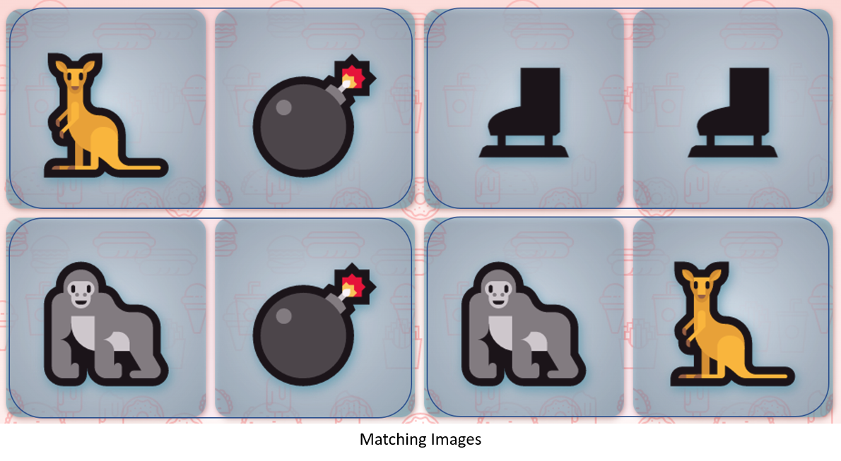
Amazingly, everything matched and I even got a matching pair on the second try. In the lower right, the first card flipped was the orangutan which I was able to match with a card seen earlier, and then the last card matched the first. So, this took six total trials to find four matches.

Eidetic Memory¶

Eidetic, or photographic memory seems to be a thing that isn't a thing. Harvard scientist Charles Stromeyer III published An Adult Eidetiker in 1970 about an artist named Elizabeth who apparently could remember images perfectly from one day to the next. The paper appears to be a hoax, though. Elizabeth was never retested, nor could anyone else demonstrate the same capability. But, let's assume we do have perfect memory.

How often should we expect to see a match to a card seen earlier? If there are $c = 2 n$ cards, with perfect memory we need no more than $c$ matches. But, let's say we've looked at $k - 1$ pairs, and flip over the first card of the $k^{th}$ pair. In the example above, maybe I would have checked the first three pairs, and on the fourth pair, the first card is the orangutan I saw in the previous pair. Instead of flipping the next card (the kangaroo), I score a point by flipping the other orangutan.

The probability the first card of the pair has a match among the previous cards is

p_1 = \frac{k-1}{c-1}

since I've seen $k - 1$ other cards already, and there are a total of $c - 1$ cards that might match the one I've just flipped over.

If there isn't a match among the cards I've already seen, there's still a small chance the first card of the pair matches the second. Since only one card matches the first one, and there are $c - 1$ other cards,

p_2 = \frac{1}{c-1}.

Letting $X$ be the required number of turns in a game, we know at most it will take $c$ turns, but we can save a few turns along the way. Since we're going to look at pairs of cards on each turn, only about half of the turns will result in a match, so I'll divide $p_1$ and $p_2$ by $2$ .

\begin{aligned} E[X] &= c - \sum_{k=1}^c \frac{p_1}{2} - \sum_{k=1}^c \frac{p_2}{2} \\ &= c - \sum_{k=1}^c \frac{k-1}{2(c-1)} - \sum_{k=1}^c \frac{1}{2(c-1)} \\ &= c - \frac{1}{2(c-1)} \sum_{k=1}^c (k-1) + 1 \\ &= c - \frac{1}{2(c-1)} \frac{c(c+1)}{2} = c - \frac{c(c+1)}{4(c-1)} \approx \frac{3}{4}c = \frac{3}{2} n. \\ \end{aligned}

The trick for calculating the sum of the first $c$ numbers is in The Sum of the Sum of Some Numbers.

Every Expectation¶

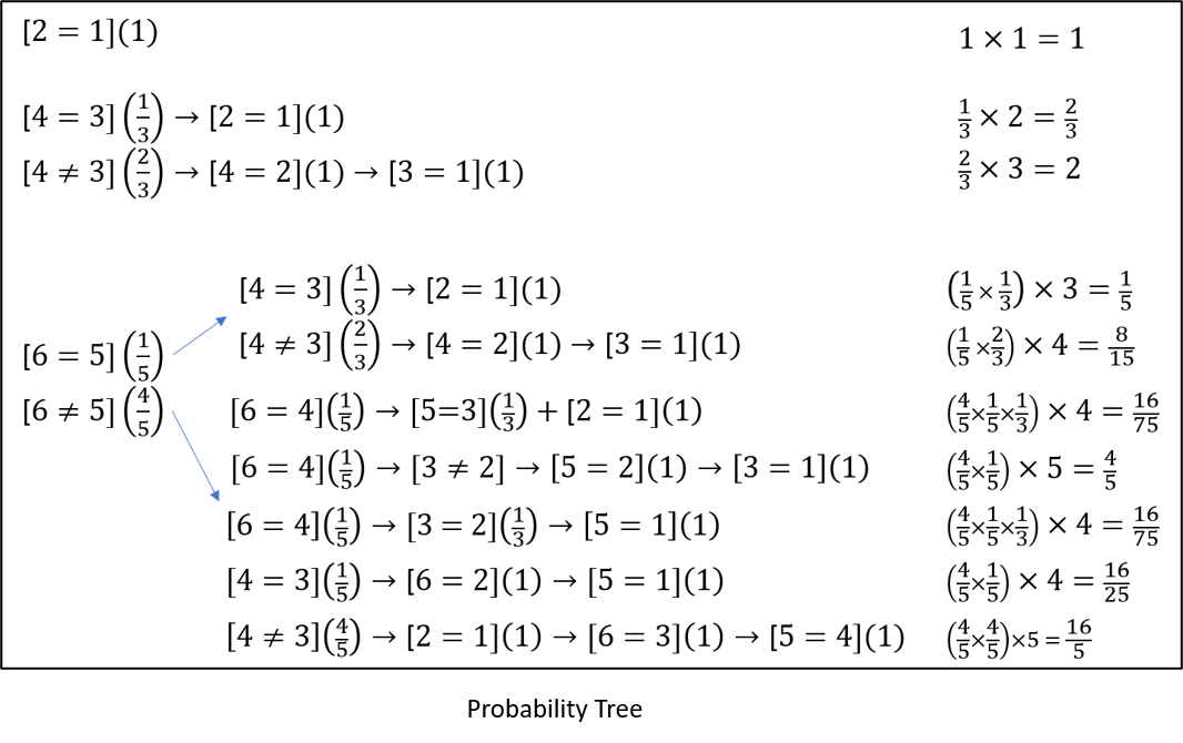
Trying to map out the possible ways a game could go gets out of hand very quickly. To analyze the play, start with a game of just two cards, and label them as ${ 2,1\}$ . The number label doesn't indicate anything about the picture on the front of the card, it's just a way to order the cards. Obviously, with only two cards in the game, they have to match and in one turn you're done.

Next, consider a game with two pairs where we'll label the cards from left to right as ${ 4,3,2,1\}$ . On the first turn, you flip over cards $4$ and $3$ . Since there are three other cards besides the first one ( $\#4$ ), the probability of getting a match on the first turn is $\frac{1}{3}$ . If you do get a match, then you'll also get a match on your second turn when you flip cards $2$ and $1$ .

The notation is $[4 = 3]$ when card $\#4$ is a match for card $\#3$ , and $\neq 3]$ when they don't match. The numbers in parentheses are the probabilities of a match.

The expected number of turns is the probability of taking a path times the number of turns, so $\frac{1}{3} \times 2 = \frac{2}{3}$ .

The more likely path, with probability $\frac{2}{3}$ , is the two cards won't match. But then you know exactly where the cards are, so you can match both in the next two turns. The expectation for this path is $\frac{2}{3} \times 3 = 2$ . The total expectation for both paths is $\frac{2}{3} + 2 = \frac{8}{3} \approx 2.667$ .

For a game with three pairs labeled ${ 6,5,4,3,2,1 \}$ , there's a $\frac{1}{5}$ probability of a match on the first turn, and then we can copy the paths we took previously. Otherwise, we need to check every possible outcome when the first two cards aren't a match. As you can see, the number of possible paths grows rapidly, and my calculations are probably wrong somewhere!

Probability Tree

A Monte Carlo Experiment¶

Imagine trying to expand the analysis to $8$ pairs, or $16$ cards! An easier way to get close to the answer is to use a Monte Carlo simulation (See The Boonie Conundrum for another example of the Monte Carlo method and how the casinos at Monte Carlo played a role in the development of the first atomic bomb.) A Monte Carlo simulation runs a random experiment many times and looks at the statistics of the outcome to get insight into a problem.

A nice feature of simulations is you can abstract away unnecessary features. By this I mean that if some part of the problem isn't needed to get your answer, you shouldn't include it in the calculation.

We'd like to know, on average, how many turns it will take to solve the Memory Game if you have Eidetic memory. As we simulate the game, we need to count turns, but we don't need to know which cards matched. If you turn over a card, there's only one other like it on the table, so the question you need to answer is, "Have I seen this card before?" Other than keeping track of where you are in the list of cards, nothing else matters.

This is an example of a game with $8$ matches, with numbers representing the icons found on the front of the cards:

{ 4, 3, 5, 8, 5, 6, 1, 8, 1, 2, 7, 6, 7, 2, 3, 4 \}.

The first turn will be used to look at the first two cards, so we can ignore it. If we have a counter called turns we can set it to $1$ , and move on. We need to keep track of the next card we'll turn over, so initialize the card counter k = 3, meaning we'll begin our game at card $\#3$ .

Have we seen card $\#3$ before? Is there a $5$ somewhere in the list before this card? If there is, we've found the one and only match for that card. The way to do this is to ask the computer,

cards[k] ∈ cards[1:k-1]

The $\in$ symbol means "in", so the code asks, "Is the $k^{th}$ card somewhere in the first $1$ to $(k - 1)$ cards?" If it is, we've found the match. If not, the match is farther down the list.

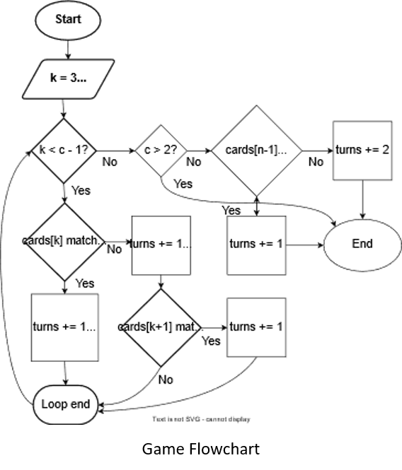
If the $k^{th}$ and $k+1)^{st}$ cards match, the turn is over and we skip forward to the $k+2)^{nd}$ card. If not, does the $k+1)^{st}$ card match one we've seen earlier? If so, take another turn and then move forward in the list.

Continue this process until you've looked at everything but the last two cards. If the last two cards are a match, you'll need one turn to look at them. If they don't you'll use one turn each to match them with cards you've seen earlier.

Here's the flowchart of the process made with the free Flowchart Maker & Online Diagram Software:

game flowchart

Put this into a loop, run it a bunch of times and you've got a Monte Carlo experiment. How many times is a "bunch"? One way to think about this is to ask how many ways can you shuffle $c$ cards? The answer is you can select the first card $c$ different ways, the second card $(c - 1)$ ways, and so on.

This is $c!$ ( $c$ factorial), but each card has an identical match so there are only $\frac{c!}{2}$ possible shuffles. For $16$ cards, there are $10461394944000$ ways to shuffle them (that's 10 quadrillion!). You need to repeat the experiment until you've sufficiently sampled the possible permutations, but I won't get into the details here.

The Results¶

I wrote the code for the Monte Carlo experiments in Julia and ran experiments using $\ldots, 16$ cards. For each experiment, I calculated how many possible shuffles there were, chose the number of Monte Carlo iterations, recorded the expected number of turns, and the expected number divided by the number of card pairs.

# cards	# shuffles	# MC	E[X]	E[X] / # matches
2	1	1	1	1
4	12	10	2.6	1.3
6	360	1000	4.559	1.519666667
8	20160	100000	6.15301	1.5382525
10	1814400	1.00E+06	7.743127	1.5486254
12	2.4E+08	1.00E+06	9.323669	1.553944833
14	4.36E+10	1.00E+06	10.91872	1.559817571
16	1.05E+13	1.00E+06	12.516	1.56449975

Using Veusz, I plotted $E [X]$ per match for each of the experiments:

shinkei-suijaku-monte-carlo

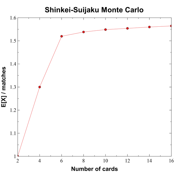
which shows the ratio is a bit over $1.5$ . For the case with four cards, $E [X] = 2.6$ , a bit lower than the analytic estimate of $2.667$ , and for six cards the Monte Carlo estimate was $E [X] = 4.559$ , while the analytic solution was $5.8$ . So, the analytic method seems to be a bit off.

From Games to Applications¶

Our analysis of Shinkei-Suijaku reveals some fascinating insights about memory, probability, and optimization. We found that random play requires about $n^2$ turns for $n$ pairs of cards, while perfect memory reduces this to approximately $1.5 n$ turns. This significant difference highlights the value of systematic approaches over random guessing - a principle that extends far beyond card games.

Try It Yourself¶

Want to explore these concepts further? Here are some experiments you can run:

Memory Strategy Testing
- Play the game multiple times using different strategies:
  - Pure random selection
  - Row-by-row systematic scanning
  - Creating mental patterns or stories to link cards
- Track your turns and completion times for each strategy
- Compare your results to our theoretical predictions
Variable Difficulty
- Modify Jan's game code to try different numbers of pairs
- Test how your performance scales with increased complexity
- Compare your scaling factor to our Monte Carlo results
Memory Enhancement
- Time yourself with and without using memory techniques
- Try describing each card aloud when you see it
- Test whether creating spatial associations improves your recall

Practical Applications¶

The principles we've explored have applications in several fields:

Education and Training
- Designing optimal flashcard systems for learning
- Creating efficient study strategies based on recall patterns
- Developing memory training programs with measurable outcomes
User Interface Design
- Organizing information for maximum memorability
- Optimizing menu layouts and icon placements
- Determining the optimal number of choices to present to users
Algorithm Development
- Improving search algorithms in databases
- Optimizing cache systems based on access patterns
- Developing better matching algorithms for various applications
Quality Control
- Creating efficient inspection patterns for manufacturing
- Developing optimal search strategies for defect detection
- Designing sampling methods for quality assurance

Future Research Directions¶

Several interesting questions remain unexplored:

How does performance change with different card arrangements (grid vs. linear)?
What's the impact of adding time pressure on strategy selection?
Could machine learning algorithms discover better playing strategies?
How do these findings translate to other memory-based games and tasks?

Our analysis of this simple memory game has taken us from basic probability to complex simulations, revealing patterns that apply far beyond the game itself. Whether you're designing educational software, optimizing search algorithms, or just trying to improve your own memory, the principles we've explored offer valuable insights into how we can systematically approach complex problems.

Remember, as Marcel Proust suggested in our opening quote, wisdom comes from our own journey of discovery. Why not start your journey by experimenting with some of these ideas? The code is available, the game is ready to play, and there's still much to learn about the science of memory and optimization.

But, enough Shinkei-Suijaku. This is your

19th-Nervous-Breakdown-Rolling-Stones

Image credits¶

Hero: Remembrance of Things Past, Marcel Proust. Midtown Scholar Bookstore.
Shinkei-Suijaku, You Win!, Matching Images: Jan De Wilde
The Rolling Stones – 19th Nervous Breakdown, Discogs

Code and Software¶

matchGame.jl - Monte Carlo simulation of the Memory Game: matchMC, playGame

Julia - The Julia Project as a whole is about bringing usable, scalable technical computing to a greater audience: allowing scientists and researchers to use computation more rapidly and effectively; letting businesses do harder and more interesting analyses more easily and cheaply.
VSCode and VSCodium - Visual Studio Code is a lightweight but powerful source code editor which runs on your desktop and is available for Windows, macOS and Linux. It comes with built-in support for JavaScript, TypeScript and Node.js and has a rich ecosystem of extensions for other languages and runtimes (such as C++, C#, Java, Python, PHP, Go, .NET). VSCodium is a community-driven, freely-licensed binary distribution of Microsoft’s editor VS Code.
Veusz - Veusz is a scientific plotting and graphing program with a graphical user interface, designed to produce publication-ready 2D and 3D plots. In addition it can be used as a module in Python for plotting.

References and further reading¶

Here are 12 references to enhance your understanding of the principles discussed in the article, focusing on both popular science articles and academic journal publications:

The Memory Game This paper delves into the classic memory game, analyzing the strategies and probabilities involved in matching pairs.
Using Monte Carlo Simulation in Game Design An exploration of how Monte Carlo simulations can be applied to game design, providing insights into balancing and probability assessments.
Monte Carlo Method: Simulation A comprehensive overview of Monte Carlo simulations, including applications in game theory and stochastic processes.
Monte Carlo Simulation Techniques An in-depth look at Monte Carlo methods, discussing their applications in various scientific fields, including game theory.
Memory and Probability This paper examines how human memory influences probability assessments, providing insights into decision-making processes.
Monte Carlo Tree Search An introduction to Monte Carlo Tree Search, a heuristic search algorithm used in decision-making processes within game theory.
The Probability of a Matching Game An analysis of the probabilities involved in matching games, offering insights into expected outcomes and strategies.
What Is Monte Carlo Simulation? IBM provides an accessible explanation of Monte Carlo simulations and their applications in various fields, including game theory.
Monte Carlo Methods for the Game Kingdomino This paper explores the application of Monte Carlo methods to the game Kingdomino, highlighting strategies and outcomes.
Time-Space Tradeoffs for the Memory Game An investigation into the computational complexities of the memory game, focusing on time-space tradeoffs.
Matching Expectations A study on the expected number of moves in the memory game, providing mathematical insights into optimal strategies.
Monte Carlo Simulation Techniques in Artificial Intelligence An introduction to Monte Carlo techniques in AI, discussing their relevance to game theory and decision-making processes.

📬 Subscribe and stay in the loop. · Email · GitHub · Forum · Facebook

The geometric distribution is a special case of the negative binomial distribution that models the number of trials needed to achieve the first success in a series of independent Bernoulli trials, where each trial has a fixed probability $p$ of success.

P(X = k) = (1 - p)^{k-1} p

where $k$ is the number of trials.

A combination is a selection of items from a larger set where order does not matter. The number of ways to choose $r$ items from $n$ is given by:

{}_n C_r = \frac{n!}{r!(n-r)!}

where $n!$ is the factorial of $n$ .

The binomial coefficient, denoted as ${}_n C_r$ or $\binom{n}{r}$ , represents the number of ways to choose $r$ elements from a set of $n$ elements without considering order. It is computed as:

\binom{n}{r} = \frac{n!}{r!(n-r)!}

It is commonly used in probability and combinatorics.

A geometric series is a series where each term is a constant multiple of the previous term. It has the general form:

ar^2 + ar^3 + \dots

where $a$ is the first term and $r$ is the common ratio. If $∣ r ∣ < 1$ , the sum of an infinite geometric series is:

\frac{a}{1 - r}

The expected value ( $E [X]$ ) of a random variable represents the long-run average outcome of a probabilistic experiment. It is calculated as:

\sum x P(x)

where $x$ represents possible outcomes and $P (x)$ is their respective probabilities.