Yacht Design with Mathematics

Home

keywords: yacht design, Bezier curves, homotopies, hull design, mathematical modeling

A ship in harbor is safe, but that is not what ships are built for.

—William Shedd

History¶

I'll show you how to design a yacht hull with five Bezier curves and a homotopy. I'll demonstrate how to make a scale model of your boat. Becoming a pirate and sailing the seven seas is left as an exercise to the reader.

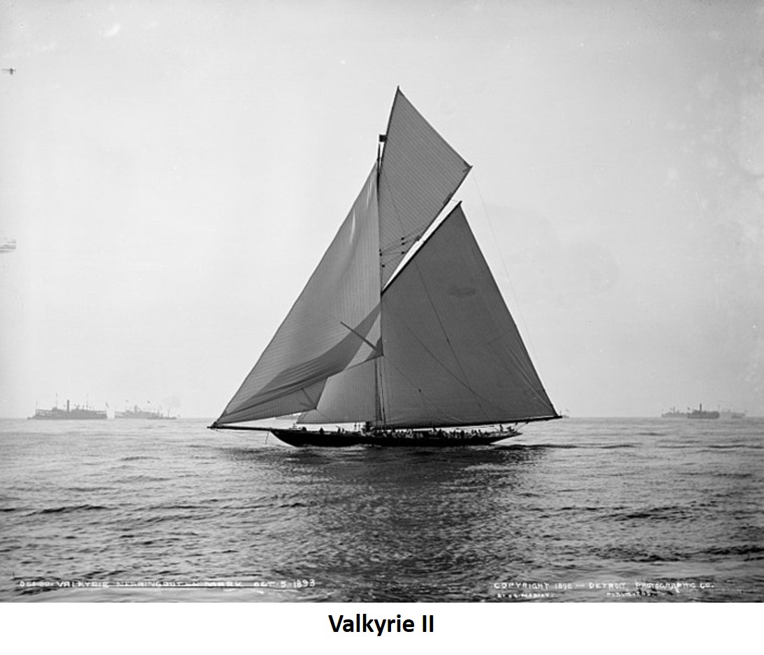
Historically, yacht designers drew the outlines of boats on their drafting boards with French curves, irregular curves, and weighted battens (or spline weights). This method produced beautiful boats, such as the British cutter Valkyrie II, the 1893 America's Cup challenger.

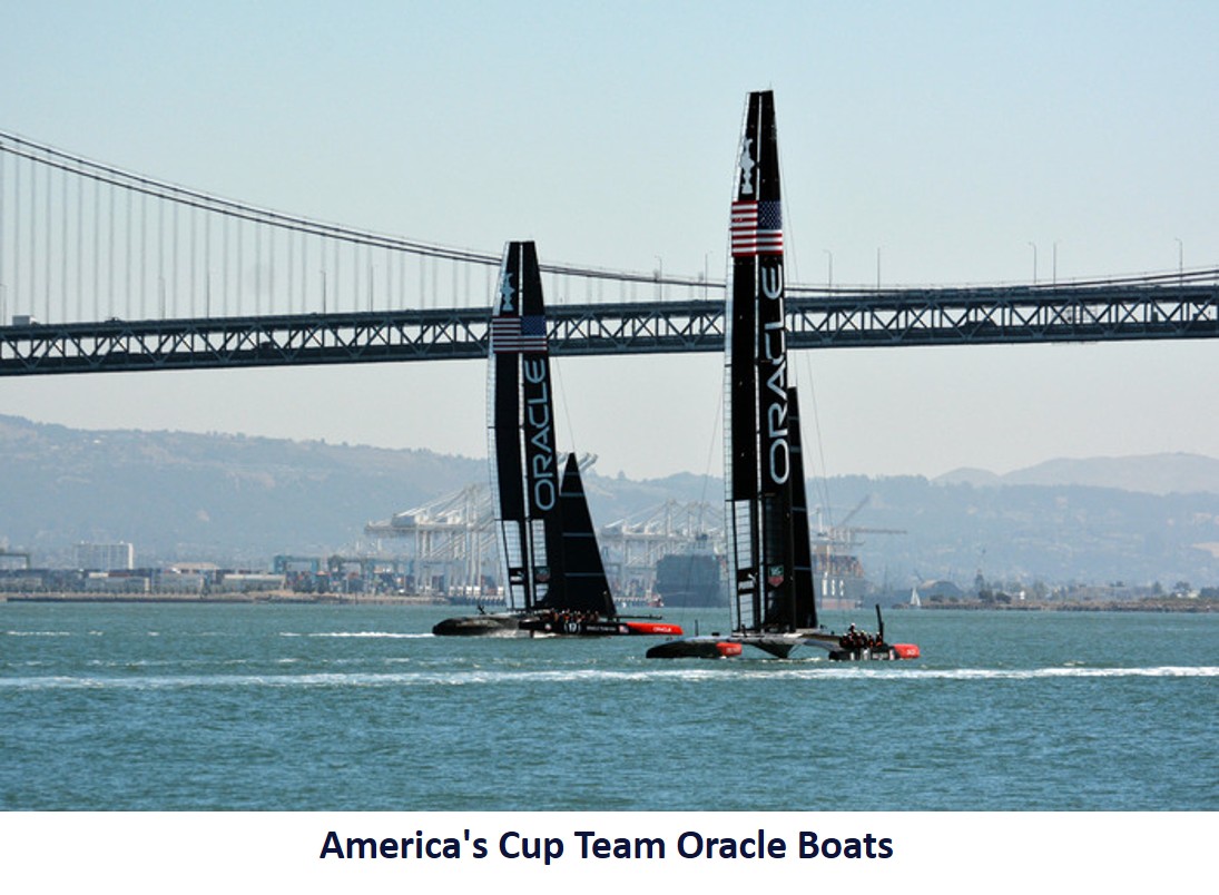
As computers became more widely available, designers turned to them to handle the difficult problems of yacht design. Now, high-performance yachts such as these by Team Oracle USA, are drawn with supercomputers calculating Computational Fluid Dynamics. In 1972, John S. Letcher published a paper, A New Approach to Numerical Fairing and Lofting, where he showed how to calculate the surface of the hull using just six curves. We can combine Letcher's method with some computer power to create the 3D shape of a hull easily. It isn't up to the level of CFD on a supercomputer, but it makes the designing process much easier than spending hours carefully drawing the outline by hand.

Letcher's Method¶

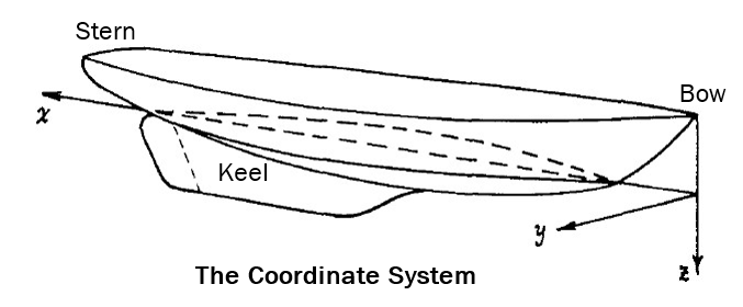
The coordinate system used by most designers starts at the bow and runs towards the stern. The origin is at the waterline directly below the bow, and positive $x$ values increase towards the stern. The lines drawings are from Letcher's paper.

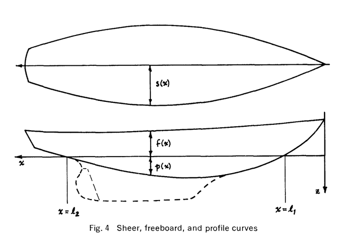
The first step is to draw the outline, which consists of three curves, the sheer $s(x)$, which is the view looking down from above, the top curve of the hull called the freeboard, $f(x)$, and the bottom without the keel called the profile, $p(x)$.

Next, the yacht is "sliced" at several points along the $x$-axis, and these section curves are typically drawn on the same plot, such as this:

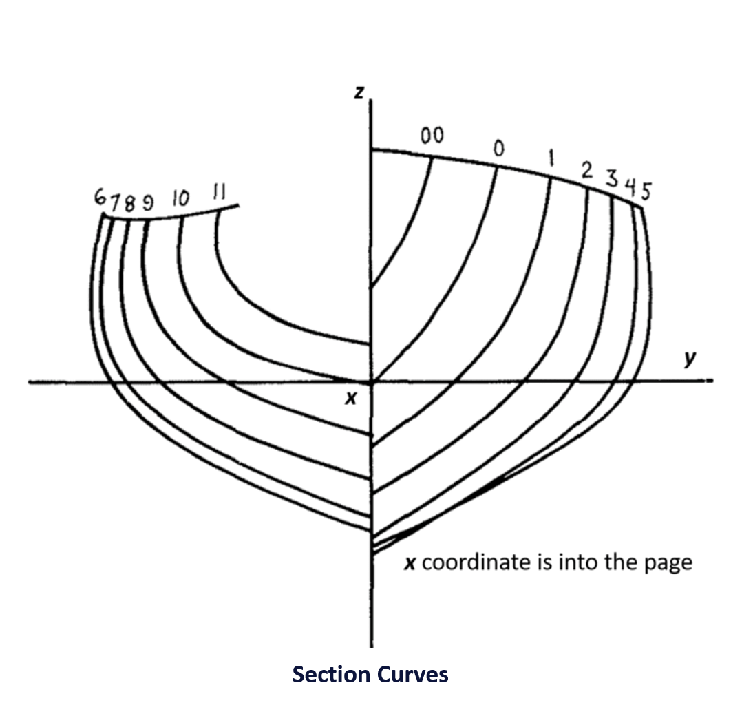
On the right side are section numbers $00,0,1,2,...,5$ looking from the bow aftwards to the maximum width. On the left side are the sections seen from the aft end looking forward. To minimize drag, the water needs to flow smoothly around this shape, so designers needed to carefully adjust the shape of each section curve (using their French curves) so there won't be any hollow areas. Designers call this "fairing".

What Letcher realized was that each of these section curves needed to be similar in shape to the ones on either side. Looking at the aft sections 9, 10, and 11 you can see they are similar, just stretched out a bit as you go from 11 to 9. Forward sections 0, 1, and 2 are also similar. So, Letcher drew two section curves, and then stretched them to meet the outline curves, sheer, freeboard, and profile.

But, how do you get a smooth transition from the aft section to the forward section? This is where homotopies come in. A homotopy is a continuous deformation of one curve into another. Letcher used the idea of homotopies to transition the section curves from the forward sections to the aft sections. Now, he had the complete design in six curves, the sheer, freeboard, profile, forward section ${\eta }_1$, aft section ${\eta }_2$, and the homotopy transition function $A(x)$.

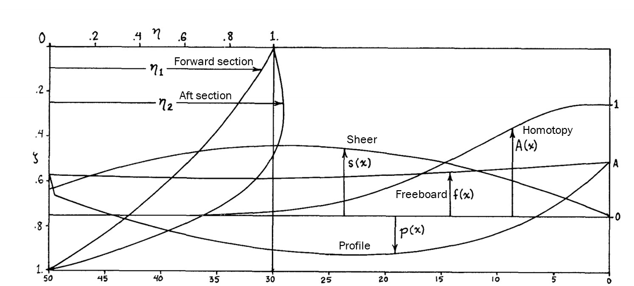
The transition function $A(x)$ varies from 1 at the bow to 0 at the stern and generates the sections from the equation

At the bow, $x=0$ and $A(0)=1$, so $\eta (x)={\eta }_1$. At the aft end, $A(x)=0$, and the section curves have transitioned smoothly to ${\eta }_2$.

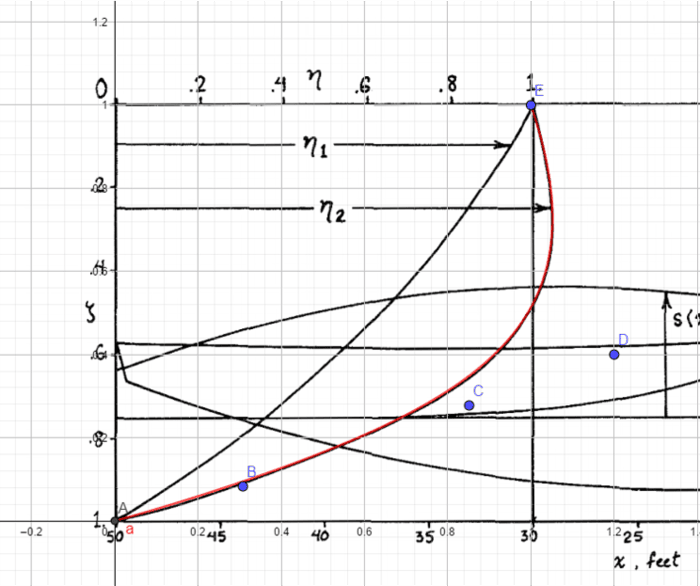
Notice the two section definition curves ${\eta }_1$ and ${\eta }_2$ are plotted in the square $(0,1)\times (0,1)$. Letcher used the coordinate system of $\eta$ as the ordinate (what we usually think of as the $x$-axis) and $\xi$ as the abscissa ($y$-axis). He also has $\xi$ increasing from top to bottom, but I'm going to switch directions for $\xi$. In our coordinate system, $x$ increases looking inward, $y$ is the horizontal axis and $z$ is the vertical axis. This violates some sacred law of coordinate systems, but I'm feeling insouciant at the moment.

To get the forward section at any $x$-axis location, we need to stretch ${\eta }_1$ until it fits the section, freeboard, and profile curves at that point. Because the sections are slices of the yacht along the $x$-axis, the section curves lie in the $y-z$ plane, and the centerline of the yacht is $y=0$. So, to stretch $\eta$ in the $y$-direction, we need to multiply by the width of the boat at each section,

The $z$ values are similarly stretched between the freeboard and profile curves. But, there's a problem. Functions are defined as the unique $z$-value at each $y$ position. Notice for ${\eta }_2$ there are two $z$-values for each $y$ for $y>1$, so ${\eta }_2$ isn't a function.

One way to handle this problem is to define the function parametrically. Think of a point traveling from one end of ${\eta }_2$ to the other in time. At time $t=0$, the point is at the lower-left corner, and at $t=1$ it's at the top right. Now, we can get both the $y$ and $z$ coordinates of ${\eta }_2$ for each value of $t$ if we know the function that transforms $t$ into positions along the curve. We'll do ${\eta }_1$ the same way, even though it could be defined as a function in the usual way.

Bezier Curves¶

Pierre Bezier invented Bezier curves when he worked at Renault during the 1960s. He used them to help draw the bodywork for cars. Bezier curves are parametrically defined polynomials shaped by a handful of control points that start and end on the first and last control points. They are defined by the $n+1$ control points $P$ as

When $t=0$,

since $0^0=1$ but $0^k=0$ for all $k>0$. Similarly, when $t=1$, $B(t)=P_n$, so the endpoints of the curve coincide with the first and last control points. Each control point $P_i=(y_i,z_i)$, are the coordinates of a point in ${\mathbb{R}}^2$ (two-dimensional coordinates), so $B(t)$ defines a curve in ${\mathbb{R}}^2$. Here's an example of a Bezier curve with five control points.

The Bezier curve (red) starts at $P_0$ when $t=0$ and ends at $P_4$ when $t=1$.

Drawing the Curves¶

We'll be using Geogebra Classic 6 to draw the curves. After you install it and start it the first time you should see a screen like this:

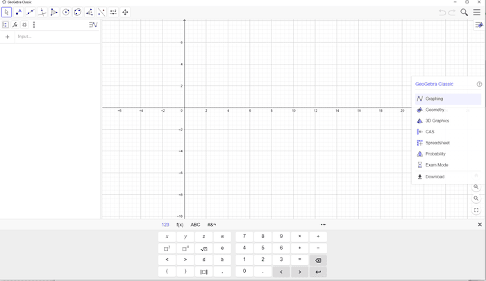
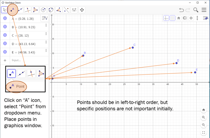
First, decide how many control points you think you might need. A few extra don't matter, but you'd like to get the curve defined with the fewest number of control points possible. For this set of curves, 5 points should be sufficient. These will be labeled A, B, C, D, and E by Geogebra. Choose the point tool from the upper left corner - an icon with a small blue dot and an "A", and select "Point" from the menu. Beginning at the origin and moving towards the right place the five points.

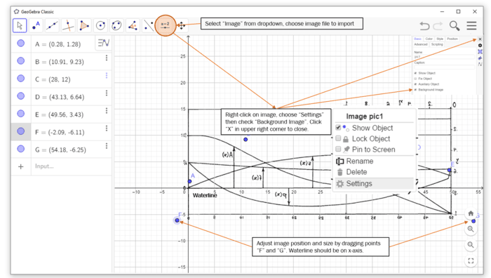
Load an image by clicking on the icon , and then choose "Image" from the dropdown menu. You may want to flip the image (in an external image editor) so the bow is on the $y$-axis. Right-click on the image to open a menu on the right side of Geogebra. Under "Basic" select "Background Image". You'll also see two points labeled "F" and "G" at the bottom left and right corners of the image. Drag these around until the image is in the correct position and scaled appropriately. The waterline should be on the $x$-axis, and the length should be 50.

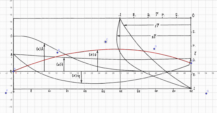
Let's start by defining the sheer curve (the one labeled $s(x)$ backward). The points "A" and "E" should be on the first and last points of the sheer curve.

On the left side, you should have the points A-E defined, and the two image control points F and G, followed by a box marked "+ Input ...". In the Input box, you need to write the Bezier equation,

You probably don't want to figure out what the equation for a 5-point Bezier curve is, so instead, run the Octave function curveString(5) which will generate the Bezier function for 5 points. Copy and paste it into Geogebra. Right-click on the dot in the function box, choose "Settings" which will open a dialog box on the right side. Select "Color" and change the color to something which stands out from the other curves (maybe red).

Now comes the fun part. First, drag the point "A" to the leftmost point of the sheer curve, and drag the point "E" to the rightmost point. Next, select one of the inner points B-D and start moving it around. Repeat with the other two until the red curve lines up with the sheer curve in the picture. Points "A" and "E" need to be exactly on the endpoints of the curve, but the others can be anywhere that gives the best fit.

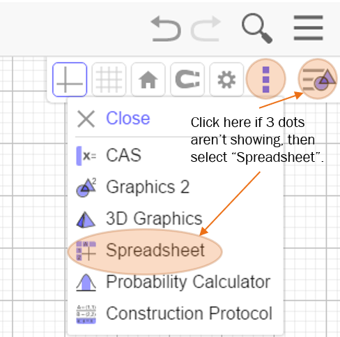
When you're done, you can export the control points to the Geogebra spreadsheet. Click on the three vertical dots in the upper right corner, and select "Spreadsheet".

You will need the following commands to copy the points into the spreadsheet. The Lst only needs to be entered once, but you need to have all of the points used, A-E, to form the curve in the list. If you used a different number of points adjust Lst, for example, if you used four points then Lst should be {A, B, C, D}.

Lst = {A,B,C,D,E}
FillColumn(1, x(Lst))
FillColumn(2, y(Lst))

Copy and paste each one of these commands into a separate Input cell in Geogebra,

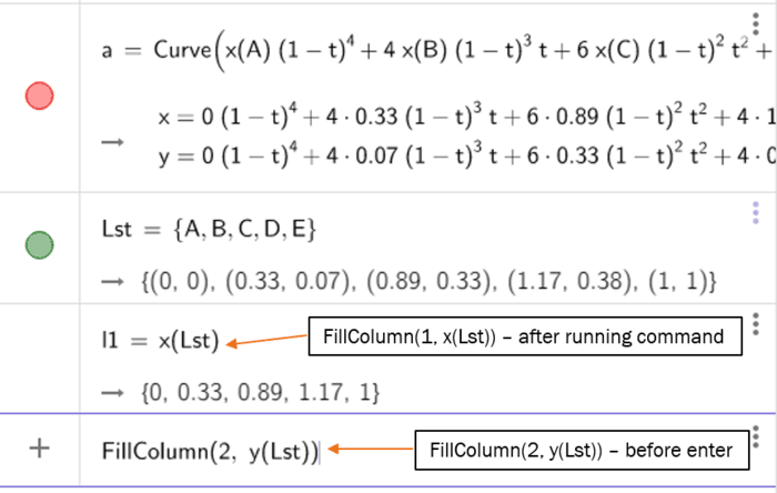
which will populate the spreadsheet:

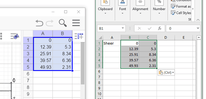
Copy the Geogebra Spreadsheet values (shown on the left above) into Excel (on the right) or Libre Office, name the curve in the first column, and repeat for the other curves: freeboard, profile, and A. For subsequent curves, just copy and paste the two FillColumn commands to update the Geogebra spreadsheet, but you won't need the Lst command again.

The two section curves ${\eta }_1$ and ${\eta }_2$ are scaled differently, so you should restart Geogebra and load the curves image again, but not flipped this time. (The image can be deleted without restarting Geogebra. See this suggestion.) This is a fit for the second section:

When you have all six curves defined, save the Excel spreadsheet.

At some point, you'll want to design your own yacht, but it's useful to have a set of curves close to what you'd like. Borrowing curves from photos or published online designs is often a good starting point. The website boatdesign is an excellent resource.

The homotopy function $A(x)$ is the least intuitive and won't show up in other designers' plans, but is also the most forgiving. How the hull transitions from one section curve to the next isn't critical to the overall plan. Letcher drew his yacht plan with the aft section ${\eta }_2$ bowing outward and then curving in towards the freeboard (called tumblehome). You can decide where you want the tumblehome to begin, and adjust $A(x)$ accordingly.

Generating Functions¶

After you have copied the control point data from each curve into the spreadsheet, save the spreadsheet to your local folder naming it something like "Letcher curves.xlsx". In Octave, open the function BezierHull and run it from the command line,

>> BezStruct = BezierHull('Letcher curves.xlsx');

where the only input is the name of the Excel file. You will need to install the Octave packages io and symbolic first. This will take a few seconds as it creates the symbolic form of each of the six curves, and evaluates them at each $x$ coordinate of the sections. Finally, it will write the sections to a text file, Letcher_curves.txt, or whatever you've named your Excel file.

If you open the file, you should find on the first line either a '1' for dimensions in feet or a '0' for meters. Below that are the coordinates $(x,y,z)$ for each of the section curves with several points along each section. You can decide how dense the points should be by setting two variables near the top of the function, dx for the separation between sections and dz for the vertical distance between waterline planes. Blank lines separate each section curve and EOF marks the end of the file.

As the function BezierHull runs, it displays the status:

>> BezStruct = BezierHull('Letcher Curves.xlsx');
Reading Excel file
Generating symbolic functions
Calculating section points
Writing points to DELFTship format file
Section points saved to Letcher_Curves.txt.
 
Length: 50.0000
Beam: 6.2647
Draft: -3.4931
Midship: 28.7693

and returns yacht parameters, Length, Beam, Draft, and Midship location from the bow. You will need these numbers for the next step.

DELFTship¶

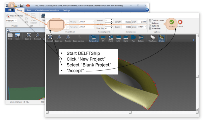
To visualize the completed hull you will need one more software tool, DELFTship. DELFTship helps naval architects design boats and ships from scratch and can provide hydrostatic, resistance, and CFD calculations, but using the Letcher method we can quickly create a yacht hull.

After starting DELFTship, click on the white rectangle in the upper left corner for "New Project" (CTRL-N) which will open a new window. In that window, select a blank project and click on "Accept".

Next to the "New Project" icon is the "Open Project" icon. Click on the down arrow and select "Import" and "Surface" (the second choice). Import the text file Letcher_curves.txt. (Notice that blanks in the file name have been changed to underscores.)

Click OK for the default number of columns, rows, and "Yes" for the dialog box, "The main particulars have not been specified",

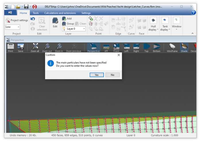
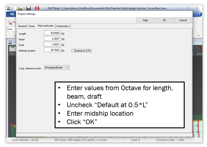
which will open a Projects Settings input. Copy the values from Octave for the length, beam, and draft (including the minus sign) and uncheck the default for midship location. Copy the values derived above, then click "OK".

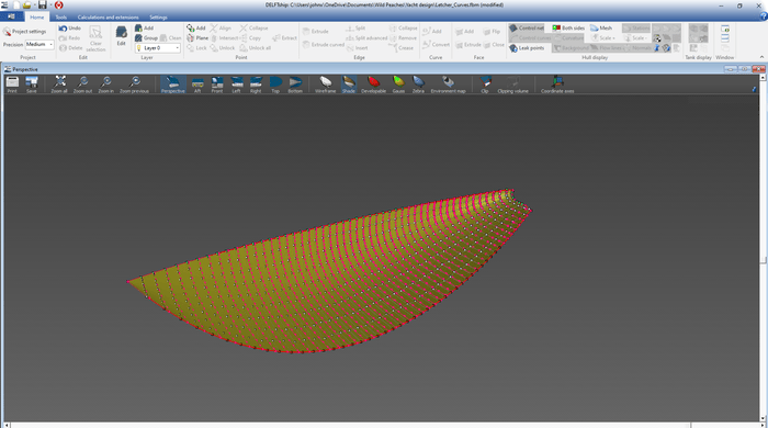
You should see the starboard half of your yacht:

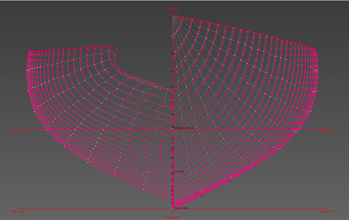
Clicking on the "Aft" and "Wireframe" icons displays the section curves similar to the ones above.

If you click on "Gauss" and "Both sides" you'll see the complete hull. Gauss indicates curvature in the hull which may be negative, zero, or positive and colored blue, green, and orange respectively. Negative curvature means locally the surface is like a saddle - it curves upwards one way and downwards in a direction perpendicular to the first. Zero curvature means that in at least one direction the surface is flat and positive means curvature is the same in both directions. For boats, the curvature should be mostly positive with possibly some flat sections. An area that shows up as blue surrounded by orange indicates the hull is not fair and will induce drag if the area is below the waterline.

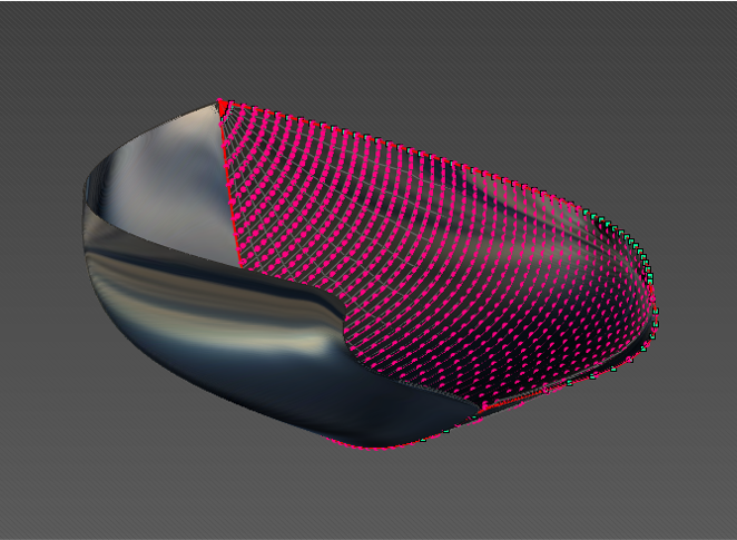
This figure shows a view of Letcher's six curve yacht from the stern with "Both sides" turned on and the "Environment map" set to "Sky". There are many more features to DELFTship you may want to explore.

Building a Model¶

You can build a model of your yacht design from styrofoam using a hot wire cutter. Jan found instructions for building a hot wire cutter from FliteTest, a group that helps amateur model aircraft builders and flyers. To use the cutter you need a rigid template attached to opposite sides of a foam block. The template guides the hot wire as it cuts through the foam, as shown here.

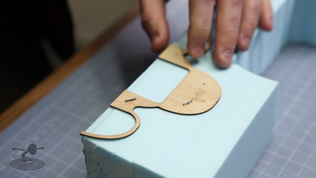
Using the sections generated from the code you can create templates for your hot wire cutter. Of course, you don't want to use templates for each cross-section, but a few along the length of the boat should be sufficient for a model. Most of the templates will be used twice during the cutting, once for each cut of adjacent blocks. After cutting all of the blocks, glue them together with a hot glue gun, and sand down the edges to smooth the surface.

Understanding the Code (TL;DR)¶

As mentioned above, you can adjust the density of points in the model by setting dx and dz. The code reads in the Excel Bezier points file for each of the six defining curves which are stored in a structure with the curve name and $x$ and $y$ coordinates of each point. The homotopy function $A$ is scaled so the $y$ values fall between 0 and 1.

Each of the six curves is converted into symbolic form with the function symBezFunc which generates terms $t_i^p$ and $(1-t{)}^{n-p_i}$ for $p_i\in 0,1,\dots ,n-1$. Multiplying each term by the binomial and Bezier control point coefficients gives the functional form,

for coordinates $x$ and $y$,

f =
 
  scalar structure containing the fields:
 
x = @(t) 50.0 * t .^ 4 + 41.09 * t .^ 3 .* (-4 * t + 4) + 170.28 * t .^ 2 .* (-t + 1) .^ 2 + 52.44 * t .* (-t + 1) .^ 3
 
y = @(t) 3.61 * t .^ 4 + 3.57 * t .^ 3 .* (-4 * t + 4) + 16.56 * t .^ 2 .* (-t + 1) .^ 2 + 15.52 * t .* (-t + 1) .^ 3 + 4.96 * (-t + 1) .^ 4

Now f can be evaluated at any value for $t\in [0,1]$,

>> f.x(0.3)
ans =  16.417
 
>> f.y(0.3)
ans =  3.8173

giving the freeboard at $x=16.417$ of $y=3.8173$ feet.

A vector, $x$, is generated at steps of $dx$ from the bow to the stern, and function funcSolve returns the value of $t$ for each $x$. This is the inverse of the previous step,

>> funcSolve(f.x,16.417)
ans =  0.30000

The $t$ values for each $x$ coordinate are stored in the function structures so section curves can be quickly evaluated. The freeboard at the $k^{th}$ section is

f.Section = f.y(f.t(k));

The section curves in $y$ and $z$ are defined as

eta.y = @(t) s.Section * (A.Section * eta1.x(t) + (1-A.Section) * eta2.x(t));

and

eta.z = @(t) (f.Section-p.Section) * (A.Section * eta1.y(t) + (1-A.Section) * eta2.y(t)) + p.Section;

With these, we can evaluate the sections at each waterline level in steps of dz.

A final section curve is generated for the transom where the $x$ values are linearly spaced between the maximum profile $x$ coordinate p.x(1) and the maximum freeboard, f.x(1). The length, beam, draft, and midship position values are calculated and displayed after the sections have been calculated.

The last step is a call to the function write2DELFTship which writes the $x,y,z$ coordinates for each section point to a text file with the same name as the input Excel file (except blank spaces are changed to underscores). If you are using meters instead of feet, change the Use_feet variable to '0' instead of '1'.

With a little bit of code modification, you could have multiple homotopies. That is, you might have three homotopy functions $A_1,A_2$, and $A_3$ with an implicit $A_4=1-A_1-A_2-A_3$, each one smoothly transitioning to the next. For each homotopy, define section curves ${\eta }_1,{\eta }_2,{\eta }_3$, and ${\eta }_4$. The requirements on the homotopies are that $0\le A_i\le 1$ and ${\sum }_{i=1}^n{A}_i(x)=1$ for all $x$.

The section curves in the yacht example start at $(0,0)$ and end at $(1,1)$ but since they are defined parametrically, any start or endpoint is possible. Using an approximately semi-circular $\eta$ could be a generating function for a submarine or aircraft fuselage. It's left as an exercise to the reader to generate a Mobius strip or Klein bottle.

Bezier curves are linear in the control point values, so it's possible to fit a set of $(x,y)$ points to an $n^{th}$ degree Bezier. Effectively, this automates the Geogebra step but requires converting a drawn curve to a set of numerical coordinates.

If you'd like to explore fluid dynamics a bit more, check out Nicole Sharp's FYFD blog. Optimizing the shape of the hull for a smooth flow could be done by adjusting the shapes of the six curves. Since they're defined using Bezier control points, a better hull shape could be generated by shifting the positions of a handful of points and running the resulting hull through DELFTship's CFD calculator or OpenFOAM.

Image credits¶

• Hero: Jürgen Venakowa, Unsplash.com
• Valkyrie II: Wikimedia Commons
• America's Cup Team Oracle Boats: CC BY-SA 3.0: D Ramey Logan, Wikimedia Commons
• Yacht line drawings: John Letcher, A New Approach to Numerical Fairing and Lofting
• Homotopy gif: Jim Belk, Wikimedia Commons
• Bezier curve: Phil Tregoning, Wikipedia
• Hot wire foam cutting: Flite Test

Code and Software¶

curveString - Generates Bezier polynomials in x and y for use in Geogebra BezierHull.m - Generate yacht hull lines using Letcher's method with all curves defined analytically using Bezier curves

• DELFTship: Yacht visual hull form modeler.
• Geogebra: GeoGebra is dynamic mathematics software for all levels of education that brings together geometry, algebra, spreadsheets, graphing, statistics and calculus in one easy-to-use package.
• LibreOffice: LibreOffice is a powerful and free office suite, with a clean interface and feature-rich tools help you unleash your creativity and enhance your productivity.
• Octave: GNU Octave is a high-level language, primarily intended for numerical computations. It provides a convenient command line interface for solving linear and nonlinear problems numerically, and for performing other numerical experiments using a language that is mostly compatible with Matlab.
• OpenFOAM: OpenFOAM is the leading free, open source software for computational fluid dynamics (CFD)

See all software used on Wild Peaches →

References and further reading¶

• A New Approach to Numerical Fairing and Lofting. John Letcher, Marine Technology Society Journal, 1 Apr 1972.
• An integrated fitting and fairing approach for object reconstruction using smooth NURBS curves and surfaces. Ali Hashemian,Seyed Farhad Hosseini, Computers & Mathematics With Applications, 30 Sep 2018.
• The Automated Fairing of Ship Hull Lines Using Formal Optimisation Methods, Ebru Narli,Kadir Sarıöz, Turkish Journal of Engineering and Environmental Sciences, 13 Jun 2004.
• Fitting Parametric Polynomials based on Bézier Control Points. Mustafa Abbas Fadhel, Recent Research in Polynomials, 11 May 2023.
• Non-linear least squares fitting of Bézier surfaces to unstructured point clouds. Joseph Lifton, Tong Liu, John McBride, AIMS Mathematics, 31 Dec 2021.
• Bezier curve interpolation on road map by uniform, chordal and centripetal parameterization. Mohd Syakir Saffie, Ahmad Ramli, AIP Conference Proceedings, 28 Jun 2018.

📬 Subscribe and stay in the loop. · Email · GitHub · Forum · Facebook

© 2020 – 2025 Jan De Wilde & John Peach