keywords: Processing, Piet, Mondrian, esoteric programming, visual coding

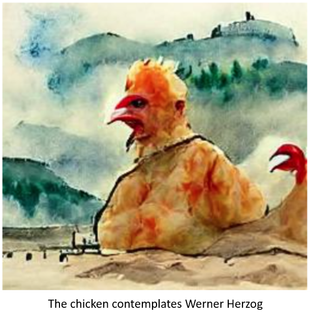
Jan is the artist of this blog. He drew the velociraptor walking on the moon for an earlier post. For anyone artistically challenged (me), computers come to the rescue. We tried using the Hotpot.ai artificial intelligence software to generate some art. The input to the program is a description of what you'd like the painting to look like. Since we'd been talking about Werner Herzog who once said,
Look into the eyes of a chicken and you will see real stupidity. It is a kind of bottomless stupidity, a fiendish stupidity. They are the most horrifying, cannibalistic and nightmarish creatures in the world.
Jan suggested "The chicken contemplates Werner Herzog" which produced this watercolor using only the text as input.
Looking around for other art-related software tools, I found two interesting programs. Processing uses the Java language to generate art, and Piet, named for the Dutch artist Piet Mondrian, uses art to create language.
Processing can create art in the style of Piet Mondrian, so I thought it might be interesting to look at Mondrian's art as both the result of computer language, and as input code.
Piet Mondrian
Piet Mondrian is considered one of the greatest artists of the 20th century. He said of art,
Art is higher than reality and has no direct relation to reality. To approach the spiritual in art, one will make as little use as possible of reality, because reality is opposed to the spiritual. We find ourselves in the presence of an abstract art. Art should be above reality, otherwise it would have no value for man.
His paintings evolved from impressionistic landscapes like Willow Grove: Impression of Light and Shadow (1905) to the abstract Composition A (1923).
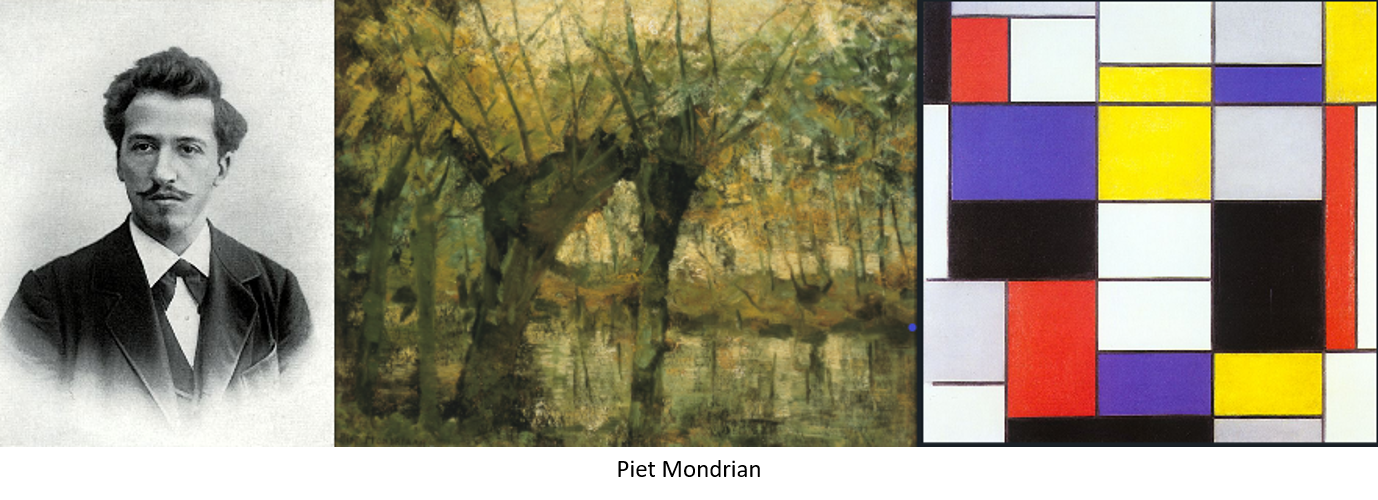
Along with other late 19th and early 20th century artists, Mondrian rejected representational art, favoring Cubism during the period 1912 - 1917, eventually settling on pure abstraction using only the primary colors red, yellow, and blue, and white, gray, and black, separated by vertical and horizontal lines.
Processing
The Processing language was started in 2001 by Casey Reas and Ben Fry in the Aesthetics and Computation Group at the MIT Media Lab. It includes an Interactive Development Environment (IDE) for writing the Java code to produce images. Programming in Processing consists of applying key terms such as background, line, ellipse, and rect with coordinate and size parameters to define location and size. Both video and written tutorials help with Processing basics.
Mondrian's Composition A makes an easy introduction to Processing because he used only six colors, and the lines are horizontal or vertical. Since I'm lazy, I thought that instead of trying to draw each line, I could paint the entire canvas black, and then paint colored rectangles on top. First, I needed to know the coordinates of each line forming the boundaries of the rectangles.
I added the Mouse_Coordinates extension for Chrome which shows the x , y x,y x,y pixel coordinates of the mouse pointer. The Piet Mondrian fan club web page lists all his paintings and has an image of Composition A where I could pick out the coordinates. I chose the right edge of each black line, using the origin ( 0 , 0 ) (0,0) (0,0) as the top left corner because both Processing and the coordinates extension use that point as the start.
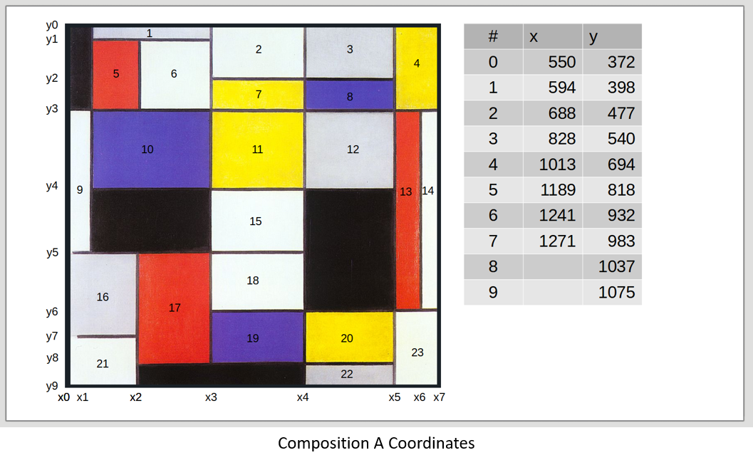
The width of the lines separating the rectangles is about 4 pixels. I numbered each rectangle to make it easier to identify in the code, so rectangle 6 lies in the region bounded by x 2 − x 3 x_2 - x_3 x2−x3 and y 1 − y 3 y_1 - y_3 y1−y3.
In the IDE, we need to tell Processing the dimensions of the image, and the color of the background, which is
0
0
0 for black. Setting rectMode to CORNERS means that we want to define rectangles by the coordinates of the corners, rather than one corner and width and height. In CORNERS mode, the first two coordinates are the upper left corner, and the next two are the lower right, corresponding to the line locations.
size(721,703);
background(0);
rectMode(CORNERS);
Next, I set the width of the lines between rectangles.
// Line width
int LW = 4;
The coordinates of the origin are ( 550 , 372 ) (550,372) (550,372), so we'll have to shift everything in Processing by subtracting x 0 x_0 x0 and y 0 y_0 y0 from the line coordinates. In Processing, we can define variables as
int left_side = 550;
int x0 = 1;
int x1 = 594 - left_side;
and so on.
We need to get the right colors for each rectangle using a color picker tool. Most paint programs like Windows Paint3D can extract color from an image, usually using an eyedropper icon. Click the eyedropper, then the color you'd like to select. The blue rectangles have a mix of colors, red 100, green 87, and blue 197.
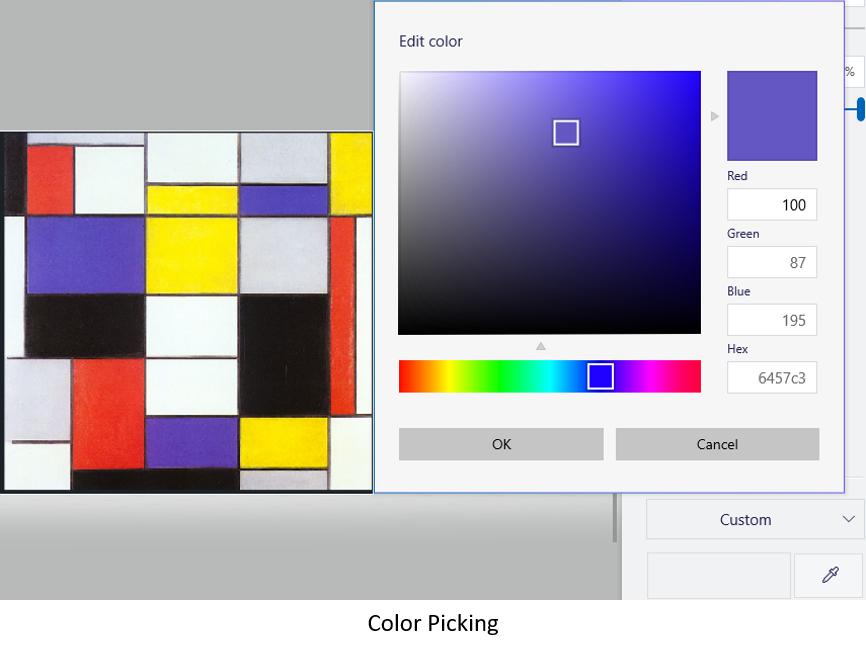
Pure red is red = 255 = 255 =255 green = 0 = 0 =0, and blue = 0 = 0 =0. Halfway between red and green is yellow, and halfway between green and blue is cyan.
Colors can be defined as variables using vector notation color(red,green,blue):
// Colors
color red = color(228,61,52);
color yellow = color(253,238,0);
color blue = color(87,70,182);
color white = color(255,255,255);
color gray = color(215,218,225);
Since we set the background color in the initialization section, we don't need a variable for black.
Mondrian's colors aren't as uniform as a single color represents, and the lines between the rectangles appear to be lighter than the black rectangles, but this will satisfy my artistic cravings.
When you start Processing you'll see the IDE with the name of the file called "sketch_<ddmmyy>a" where "ddmmyy" is today's date. Start writing your code on the first line.
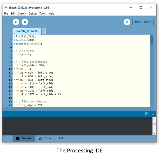
Notice that two forward slashes // start a comment. Also, the location of the last
x
x
x line, x7 is the pixel location (1271) minus the left_side plus the line width LW. Later, we'll define the width and height of each rectangle as the line locations minus the widths, but to get the full extent of the image the line width needs to be added back.
Rectangles with an edge on either the left side or top of the image should have that coordinate set to 1 1 1 meaning that it starts in the first pixel. I redefined x 0 = 1 x0 = 1 x0=1 and y 0 = 1 y0=1 y0=1 for consistency while making the rectangles.
Each rectangle can be defined by the lines that surround it, and the color by the fill command,
// Rectangle #1
fill(gray);
rect(x1,y0,x3-LW,y1-LW);
Continue building the remaining rectangles. Save the file (sketch_220624.pde), and then press the Run button at the top of the edit area of the IDE (the blue triangle in a white circle). If all goes well you should have a perfect reproduction of Composition A.

The basic unit of code in Piet is a codel, the smallest square of color used. It's like a pixel, but to make a codel visible, they're usually many pixels across. The gray rectangle in the top left (block #1) is contained between x 1 = 44 x1 = 44 x1=44 and x 3 = 278 x3 = 278 x3=278 and y 0 = 1 y0 = 1 y0=1 and y 1 = 26 y1 = 26 y1=26. The length is 234 pixels and the height is 26 making the width 9 times the height. If we define a codel to be 26 × 26 26 \times 26 26×26 pixels, then the gray block is 9 × 1 9 \times 1 9×1 codels.
Every computer language needs to know how to "read" the code. For Piet, the starting point is always in the upper left corner, which would be a black codel. Piet uses two different pointers to control the direction of travel through the program. The Direction Pointer (DP) initially points to the right and is the direction taken until it reaches the edge of a color block. The direction can be right, left, up, or down.
The Codel Chooser (CC) selects the edge of the current codel which can be either the left or right edge. The starting value for the CC is left, and the values for both the DP and the CC change frequently during the program execution. The rules for moving through the code are
- The interpreter finds the edge of the current color block which is furthest in the direction of the DP. (This edge may be disjoint if the block is of a complex shape.)
- The interpreter finds the codel of the current color block on that edge which is furthest to the CC's direction of the DP's direction of travel. (Visualize this as standing on the program and walking in the direction of the DP.)
- The interpreter travels from that codel into the color block containing the codel immediately in the direction of the DP.
After this, the rules get more complicated than The Campaign for North Africa. Imagine the colors, excluding white and black, wrapped around a cylinder. Next, bend the cylinder around a circle to form a torus like the image of Earth at the top. The Earth isn't flat, it's a torus. Just ask Neil deGrasse Tyson.
The magentas on the right end are connected to the reds on the left end, and the light colors are connected to the dark. Depending on color and intensity changes between adjacent codels, the Piet interpreter will perform different actions.
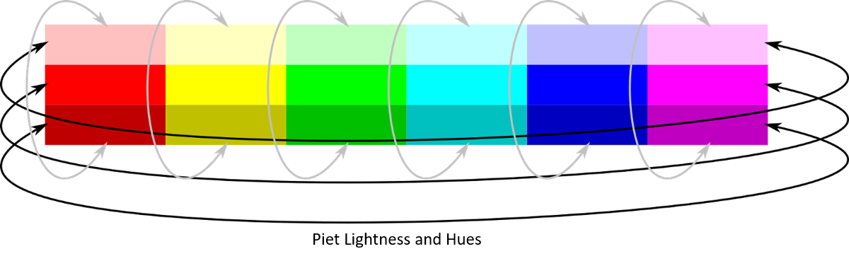
Suppose you're on a medium yellow and move onto a dark blue. That's 3 steps in hue and one in intensity. If your next move is to the light green, then you've gone 4 steps in hue and 1 in intensity. Depending on how many steps you make, a different rule applies.
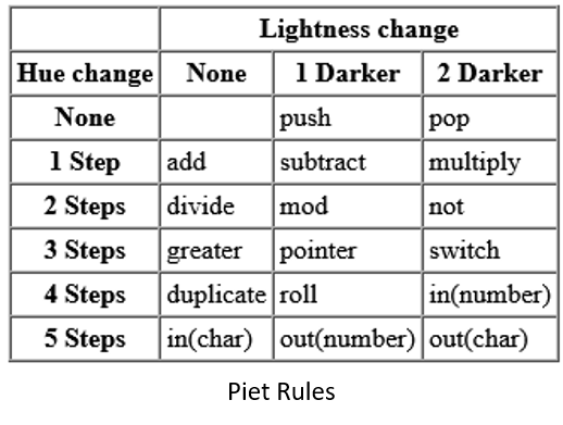
Dark blue to normal green is 4 steps in hue and 1 in intensity which is roll. Even though the move is from dark blue to light green, it's 1 Darker because you're wrapping around the torus in the clockwise direction if you're looking down the tube from the red end.
roll: Pops the top two values off the stack and "rolls" the remaining stack entries to a depth equal to the second value popped, by a number of rolls equal to the first value popped. A single roll to depth n is defined as burying the top value on the stack n deep and bringing all values above it up by 1 place. A negative number of rolls rolls in the opposite direction. A negative depth is an error and the command is ignored. If a roll is greater than an implementation-dependent maximum stack depth, it is handled as an implementation-dependent error, though simply ignoring the command is recommended.
So that's clear. The stack is the computer memory. It's like a stack of paper where you can write one number or character on a piece of paper, and then "push" it onto the top of the pile. To get the number back, you "pop" it off the top of the stack. You can only pop one number at a time, and only the top number on the stack.
The computer can do basic arithmetic - add, subtract, multiply and divide. It does this by popping the top number off the stack, popping the next one, adding the two together, and pushing the result back onto the stack. Five color changes and two darker pops a character from the stack. Even though all data on the stack are integers, the command out(char) prints the ASCII equivalent of the top number on the stack. A 65 becomes "A", 90 is "Z", 97 is a lower case "a", and 122 is "z".
More detailed instructions for programming in Piet are available from these sources:
- The official Piet page by David Morgan-Mar (aka Dangermouse)
- Fun with Piet article on Medium by Katharina Sick
- The Esolangs Wikipage for Piet
- Manfred Moosleitner's Piet - An Artistic Programming Language
- The npiet pages with an example program trace
- Marc Majcher's description of the language
- Gabrielle Singh Cadieux's slides of her MasterPiets IDE
MasterPiets
I think the easiest way to get acquainted with Piet would be to read David Morgan-Mar's page, and then skip right to the end of the list above and go through Gabrielle Singh Cadieux's presentation. MasterPiets is her implementation of the Piet interpreter and it runs in a browser window, so you don't need to download anything.
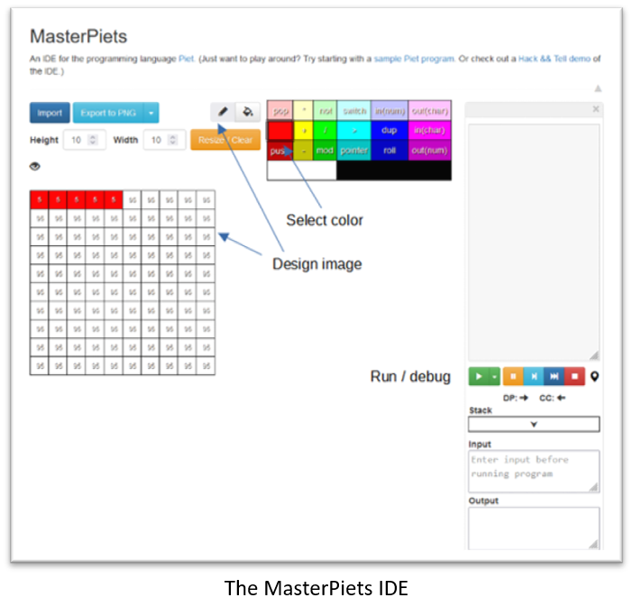
Everything you need is built-in. Decide how big you want the image to be, and set the height and width. Click on the eye to display the number of codels in each block. Select a color and the pen icon to begin filling in individual blocks. When you've finished, click the green run button, or if you want to debug your code, pause with the orange button, step with light blue, or set breakpoints and run to the break using the dark blue arrow.
Let's jump right in and try to code something. Many beginning programs start by printing "Hello World", which Gabrielle has included in her slides. A slight modification could be "Welcome" for your front door welcome mat. The ASCII code for "W" is 87, so we could create a block with area 87, push it onto the stack, and then use the "out(char)" command to get "W" in the output window.
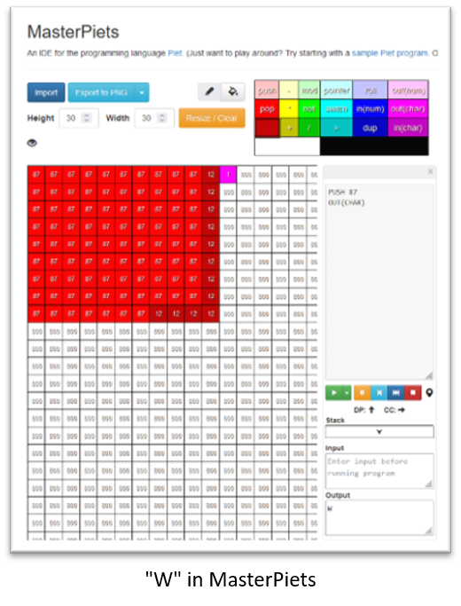
I filled in an area of 87 squares in red, then made a few blocks to the right in dark red ("push") and finally made one square magenta for "out(char)". Clicking the green run button pushes 87 onto the stack and then writes the character "W" in the output window.
A very nice feature of MasterPiets is that when you select a color to fill in your block, the commands get rearranged in the color selection window so you know which color you need for the next command. From red, I needed dark red to "push", and then to get the "W" in the output window, I need magenta.
Mondrian rectangle statistics
I wanted to create a painting in the spirit of Mondrian by making the blocks rectangular, but the factors of 87 are 3 and 29 which would make a skinny rectangle. The letter "e" is 101, a prime number giving a rectangle 1 × 101 1 \times 101 1×101.
If you look at the rectangles from several of Mondrian's Compositions (2, C, II, III, with red and blue, with blue, with gray and light brown), and compare width to height (taking the larger value as the numerator) a histogram of the ratios is:
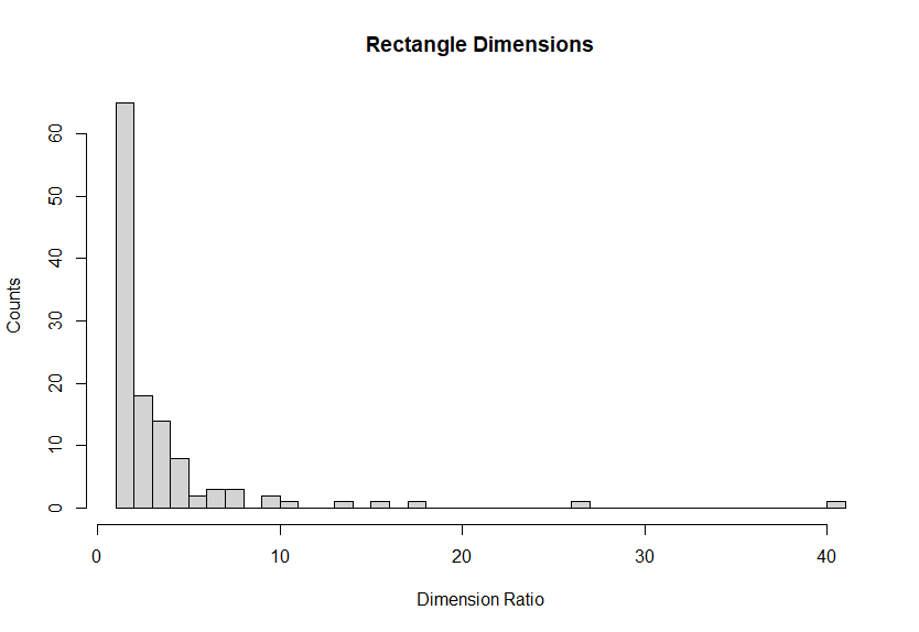
To make Piet seem more Mondrian, we should make rectangles that represent the distribution of ratios found in his original paintings. There are many probability distributions, so we need to find one that fits the data. A distribution is a mathematical function that describes the probability of an event occurring under certain conditions.
For example, if you roll a die, the probability of getting any one of the six possible numbers is presumed equally likely. The distribution describing this is called the Uniform distribution. Another distribution you may have seen is the Normal distribution with the familiar "bell-shaped" curve. But, the data from 121 Mondrian rectangles isn't either of those two distributions.
Using R, it's possible to estimate a good fit to the data. First, read in the data. Next, plot the empirical density and cumulative distribution:
rectDims <- read.csv("../rectangle-dimensions.csv")
library(fitdistrplus)
plotdist(rectDims$Ratio, histo = TRUE, demp = TRUE, breaks = 40)
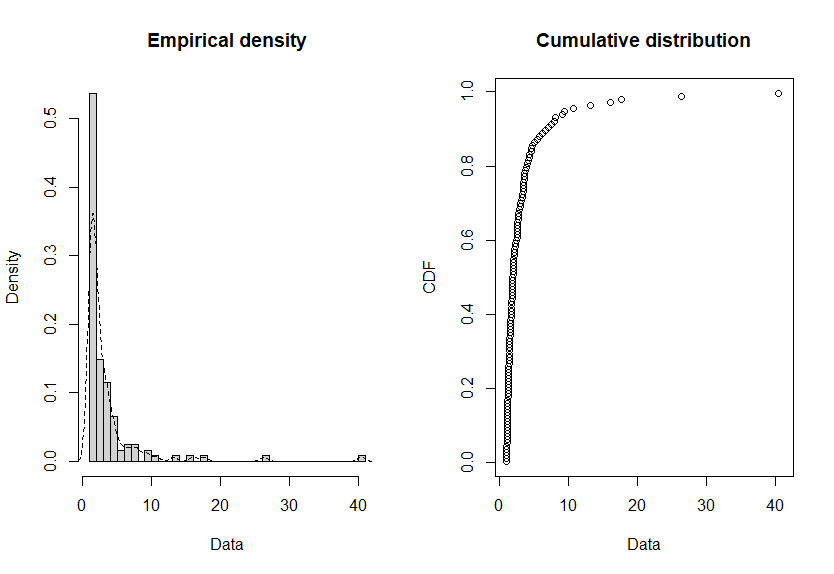
The dotted curve in the Empirical density plot is the function we'd like to approximate. Applying the function descdist,
descdist(rectDims$Ratio, discrete=FALSE, boot=500)
summary statistics
------
min:  1   max:  40.375
median:  1.901961
mean:  3.432443
estimated sd:  4.88203
estimated skewness:  4.998436
estimated kurtosis:  34.11326 r
gives basic statistics about the data. Skewness indicates how the data tends to be displaced to one side or the other of the maximum
Skewness = ∑ i = 1 N ( X i − μ ) 3 / N σ 3 . \text{Skewness } = \frac{\sum_{i=1}^N (X_i - \mu)^3/N}{\sigma^3}. Skewness =σ3∑i=1N(Xi−μ)3/N.In the summary statistics, the standard deviation, σ \sigma σ is labeled "estimated sd", and the mean is μ \mu μ in the equation.
If you flatten or pull up a normal distribution, you've got kurtosis and should seek medical advice immediately.
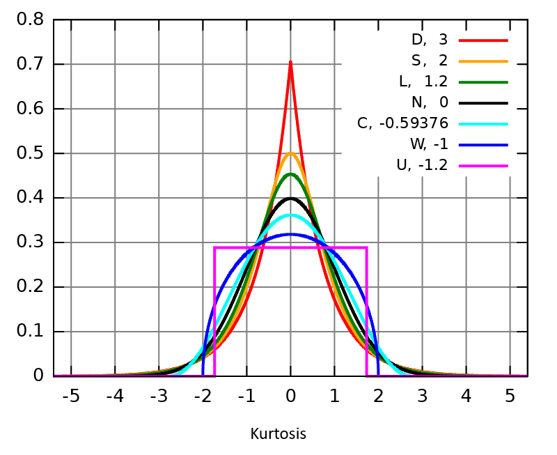
The red curve has large kurtosis, while the magenta curve is low. The formula for kurtosis is the same as skewness, except that the exponents are 4 4 4 instead of 3 3 3.
The Mondrian rectangles are strongly skewed to the right side and have a sharp peak at
1
1
1, so the kurtosis is very high as well. The descdist function produces a Cullen and Frey graph
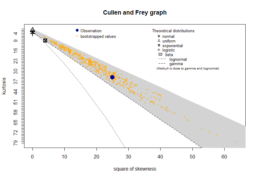
showing how well the data matches several other distributions. The blue dot at (25,34) is the observed data from the Mondrian rectangles. The yellow diamonds are bootstrap samples generated using a Monte Carlo resampling of the original data. An Introduction to the Bootstrap by Efron and Tibshirani is a good resource.
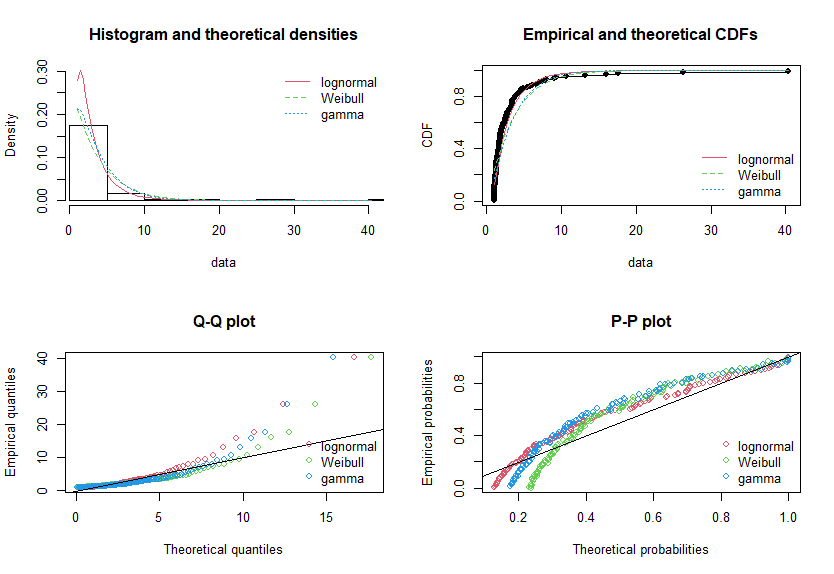
Both the observational data and the bootstrap values fall into the region covered by the beta distribution, so that seems like a good initial guess. But, if we fit log-normal, Weibull, and Gamma distributions, it looks like the log-normal gives the best fit
using the commands
# Estimate distribution parameters
fitRect <- list()
fitRect$lnorm <- fitdist(RR,"lnorm")
fitRect$weibull <- fitdist(RR,"weibull")
fitRect$gamma <- fitdist(RR,"gamma")

# Plot fits
par(mfrow=c(2,2))
plot.legend <- c("lognormal", "Weibull", "gamma")
denscomp(fitRect, legendtext = plot.legend)
cdfcomp (fitRect, legendtext = plot.legend)
qqcomp  (fitRect, legendtext = plot.legend)
ppcomp  (fitRect, legendtext = plot.legend)
Summary statistics for the log-normal distribution are returned using
> summary(fitRect$lnorm)
Fitting of the distribution ' lnorm ' by maximum likelihood
Parameters :
         estimate Std. Error
meanlog 0.8492164 0.06761462
sdlog   0.7437608 0.04781037
Loglikelihood:  -238.6264   AIC:  481.2528   BIC:  486.8444
Correlation matrix:
              meanlog         sdlog
meanlog  1.000000e+00 -2.296957e-11
sdlog   -2.296957e-11  1.000000e+00
which says that the mean of the log-normal fit is μ = 0.8492164 \mu = 0.8492164 μ=0.8492164 and the standard deviation is σ = 0.7437608 \sigma = 0.7437608 σ=0.7437608. As a check, plot the log-normal distribution using the fitted parameters,
curve(dlnorm(x, meanlog=0.8492164, sdlog=0.7437608), from=0, to=40)which should have the same shape as the red curve in the Histogram and theoretical densities plot above.
I doubt Mondrian took this much trouble to define the distribution of the sizes of his rectangles, but if we generate random rectangles from this distribution, it will seem more Mondrian-like.
Generating the rectangles
Looking at the ASCII table, the codes corresponding to each letter are
| Letter | W | e | l | c | o | m | e |
|---|---|---|---|---|---|---|---|
| ASCII | 87 | 101 | 108 | 99 | 111 | 109 | 101 |
Letter "W" needs 87 blocks, which could be either
1
×
87
1 \times 87
1×87 or
3
×
29
3 \times 29
3×29. But, if we're willing to relax the requirements a little, we can generate a few random log-normal distributed numbers using rlnorm,
nIter <- 5
meanlog <- 0.8492164
sdlog <- 0.7437608
rlnorm(nIter,meanlog,sdlog)
[1] 4.4361233 2.8549616 0.8354034 1.1958887 8.1149446
Using the first random number, we'd like to make a rectangle with sides x x x and y y y such that x × y = 87 x \times y = 87 x×y=87 and x = 4.4361233 × y x = 4.4361233 \times y x=4.4361233×y. Let's call the random number r r r, and the ASCII representation of "W", n = 87 n = 87 n=87. Then
x y = n y = x r x 2 r = n x = r n \begin{aligned} xy &= n \\ y &= \frac{x}{r} \\ \frac{x^2}{r} &= n \\ x &= \sqrt{rn} \end{aligned} xyyrx2x=n=rx=n=rnSince the random number r r r isn't likely to be a whole number, and the square root of r × n r \times n r×n isn't either, then we need to round x x x to the nearest integer. To get y y y, divide x x x by r r r, and round to the nearest integer. This leaves a remainder, so we'll have to make a small rectangle to be added to the first.
Rather than calculating the values for
x
x
x and
y
y
y for each letter, the function printRects prints several possible combinations of rectangle dimensions, and the associated remainder.
inStr <- "Welcome"
nIter <- 5
meanlog <- 0.8492164
sdlog <- 0.7437608
printRects(inStr,nIter,meanlog,sdlog)
[1] "W"
[1] "(x,y) = [13, 6], rmdr = 9"
[1] "(x,y) = [9, 8], rmdr = 15"
[1] "(x,y) = [17, 4], rmdr = 19"
[1] "(x,y) = [14, 5], rmdr = 17"
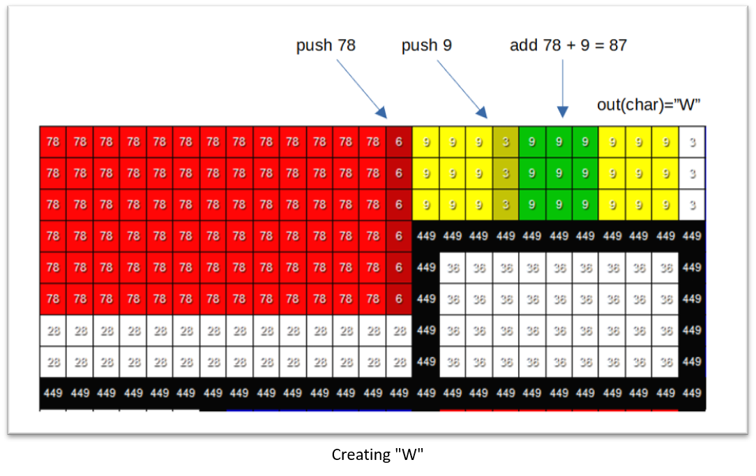
[1] "(x,y) = [15, 5], rmdr = 12"For "W" we could make a 13 × 6 = 78 13 \times 6 = 78 13×6=78 rectangle, followed by a 3 × 3 = 9 3 \times 3 = 9 3×3=9 rectangle. The code in Piet would be
push(78)
push(9)
add
out(char)
The reason for asking the function to give several possible combinations is that the remainder might be prime as in the 3 r d 3^{rd} 3rd and 4 t h 4^{th} 4th cases, which would require a 1 × 19 1 \times 19 1×19 or 1 × 17 1 \times 17 1×17 rectangle. Since the code reduces the value of x x x by 0.9 0.9 0.9, sometimes the remainder works out to be one of the two dimensions of the rectangle. In that case, you can increase the length of the other side.
The rectangle dimensions I chose were
| Letter | W | e | l | c | o | m | e |
|---|---|---|---|---|---|---|---|
| ASCII | 87 | 101 | 108 | 99 | 111 | 109 | 101 |
| x | 13 | 11 | 12 | 11 | 12 | 11 | 9 |
| y | 6 | 8 | 9 | 9 | 8 | 8 | 9 |
| rx | 3 | 13 | 0 | 0 | 5 | 7 | 5 |
| ry | 3 | 1 | 0 | 0 | 3 | 3 | 4 |
where r x rx rx and r y ry ry are the dimensions of the remaining rectangle. The sum of the ASCII values is 716, and we'll need more for the commands, but give yourself room for artistic creativity.
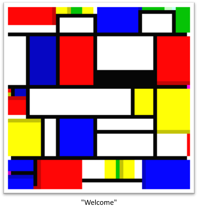
To make the letter "W", I made a block of 13 × 6 = 78 13 \times 6 = 78 13×6=78 in red, followed by dark red "push", a 3 × 3 = 9 3 \times 3 = 9 3×3=9 yellow block, and another "push" in dark yellow. Next, I put in a green block for "add" and finished with a yellow "out(char)". Here are the details:
The sizes of the "push", "add", and "out(char)" blocks can be anything, so sometimes I used a single codel at the end of a black line. White codels pass the pointer on to the next color block without changing anything. I found that putting in some white in the code helped keep track of which blocks belonged together to create a single letter.
The code starts in the upper left corner (the red block), travels across the top, down the right side, across the bottom, and then up the left side until it hits a solid black line where it stops. Much of the interior is never accessed, so you can put anything you like in that region.
The output from this code is shown in the MasterPiets Output window:
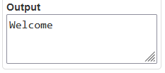
I input Mondrian's Composition A into MasterPiets and it spits out some nonsense, "daed si luaP". I have no idea what that's about.
The future of art
By changing the size of the painting, the colors used, and the size of the codel blocks, the same output can be generated in many vastly different formats. The colors used in Piet aren't entirely Mondrian, but you can get close to the original Mondrian style if you're careful. Thomas Schoch wrote this Piet program that spells "Piet" when run.
Piet is a Turing complete language which means it can simulate any other Turing complete language. In principle, you could write a Piet program that would output a Processing sketch that would look like the original Piet program.
Piet isn't limited to simply printing words, either. On David Morgan-Mar's Piet Program Gallery you'll find Clint Herron's implementation of Euclid's Algorithm for calculating the greatest common divisor of two integers. We discussed Euclid's Algorithm in Haven's Haven.
Artists of Mondrian's time were the Avant-Garde or Modernists. By the middle of the 20th century, art became post-modern, and by the end of the century, post-post-modern, post-millennial, post-mondrian, or post-malone*. With computers and specialty esolangs we have now entered the era of pre-futurism.
* Post Malone's real name is Austin Richard Post, but he used an online rap name generator for his first mix tape. Jan's rap name is Wilde Da Baby and mine is lil' peachfuzz.
Image credits
Hero: Apparently, Some People Believe the Earth Is Shaped Like a Donut. Beckett Mufson,Vice, Nov. 13, 2018.
The chicken contemplates Werner Herzog: Jan De Wilde and John Peach. Hotpot.ai
Piet Mondrian: Wikimedia Commons
Willow Grove: Impression of Light and Shadow: Wikimedia Commons.
Composition A: Happy Birthday Mondrian!. Lon Levin, The Illustrators Journal, Mar 7, 2012.
Code and Software
mondrianRects.r - Generate Mondrian dimensional rectangles from ASCII characters of input string.
rectangle-dimensions.csv - Dimensions of rectangles from several Mondrian paintings.
- Processing - is a free graphical library and integrated development environment (IDE) built for the electronic arts, new media art, and visual design communities with the purpose of teaching non-programmers the fundamentals of computer programming in a visual context.
- Piet - Piet is a programming language in which programs look like abstract paintings. The language is named after Piet Mondrian, who pioneered the field of geometric abstract art.
- MasterPiets - An IDE for the programming language Piet.
- R and RStudio - R is a language and environment for statistical computing and graphics. RStudio is an integrated development environment (IDE) for R. It includes a console, syntax-highlighting editor that supports direct code execution, as well as tools for plotting, history, debugging and workspace management.
References and further reading
- Processing: A Programming Handbook for Visual Designers and Artists This comprehensive book by Casey Reas and Ben Fry introduces the Processing programming language, exploring its applications in visual design and art.
- Piet: A Language for the Eye David Morgan-Mar's official page on Piet provides an overview of this esoteric programming language, where programs are abstract images resembling the works of Piet Mondrian.
- Processing: Creative Coding and Computational Art Ira Greenberg's book offers insights into creative coding using Processing, blending programming with computational art.
- Generative Design: Visualize, Program, and Create with Processing This book by Hartmut Bohnacker and colleagues delves into generative design principles using Processing, providing practical examples and techniques.
- Esoteric Programming Languages: Piet The Esolang wiki offers an in-depth look at Piet, discussing its design principles and providing examples of programs.
- Creative Coding: Aesthetic Computing This chapter explores the intersection of creative coding and aesthetic computing, highlighting how programming can be an artistic endeavor.
- The Art of Creative Coding A PBS segment that showcases artists and designers who use code as their creative medium, illustrating the possibilities of creative coding.
- Processing Community The official Processing community page connects users to forums, exhibitions, and resources, fostering a collaborative environment for creative coders.
- Piet Mondrian: The Complete Works A comprehensive collection of Piet Mondrian's artworks, providing context to the visual style that inspired the Piet programming language.
- Algorithmic Art: Combinatorics and Visual Creativity This article discusses the role of algorithms in art creation, emphasizing combinatorial methods and visual creativity.
- openFrameworks: An Open Source C++ Toolkit for Creative Coding An open-source C++ toolkit designed for creative coding, offering tools for artists and developers to create interactive projects.
- The Processing Foundation The foundation behind Processing, dedicated to promoting software literacy within the visual arts and visual literacy within technology.
📬 Subscribe and stay in the loop. · Email · GitHub · Forum · Facebook
© 2020 – 2025 Jan De Wilde & John Peach