keywords: genetic algorithms, Procrustes method, bin packing, yacht design, computational modeling
Flites of Fancy
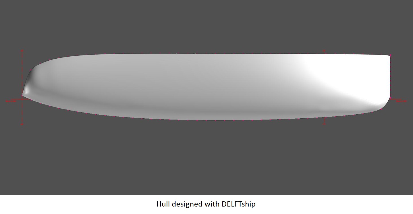
Building a model helps to get a feel for how the ideas developed in the previous posts Betz The Limit and The Pushmi-Pullyu might work. A catamaran (see Of Sailing Ships, Velociraptors, and Walking on the Moon) provides a relatively steady surface to attach the wind turbine. For this model, I ignored detailed calculations but used the method described in Yacht Design with Mathematics to create the hull form.
To keep the hull relatively simple, the freeboard (top edge of the hull) is a straight line except where it tapers at the stern.

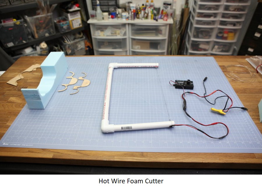
The people at Flite Test put out lots of great videos showing how to create model aircraft and one of their videos shows how to make a hot wire foam cutter,

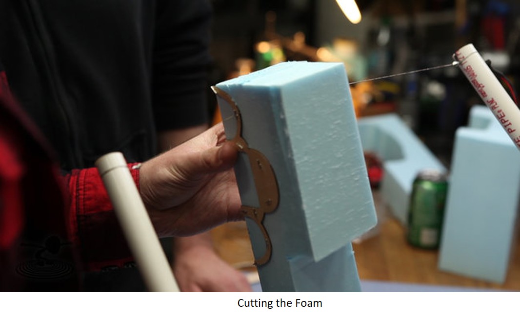
and how to build templates to create the shape.

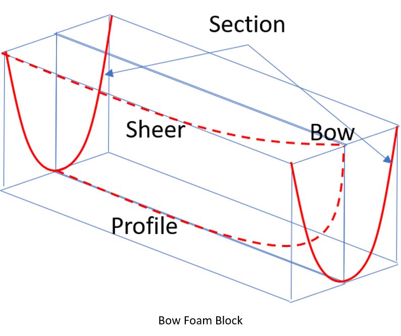
The mathematical tools shown in the yacht design post can easily be modified to create the JA 37 Viggen jet shown in their video by modifying the shape of the section curves, and possibly using more than one homotopy, but for this project that's not necessary. A few section curves along the length of the hull, and sheer and freeboard/profile curves at the bow and stern should be sufficient. Here's a plot of the curves drawn in Octave,

The top two rows are sections while the bottom row (from left to right) shows the half-bow sheer, half-stern sheer, bow freeboard and profile back to the first section, and the freeboard and profile for the aft section. The reason for using only half the sheer curve is that the sheer and freeboard/profile curves can be combined at right angles on a piece of foam to cut the bow and stern pieces. It might be useful to first cut the general outline by using two copies of the first and last sections.
To make the bow, make two rectangular blocks of foam that are half the width of the boat at the first section, as deep as that section, and the length of the distance between the bow and the first station. Attach a copy of the section template at both ends and use the hot wire cutter to generate the hull shape at the section curve.

Separate the two pieces of foam, and attach the sheer curve template to the top, and the profile to the inner edge. Now use the hot wire cutter to remove the excess foam to shape the bow, and glue the two pieces together. The same process can be done at the stern.
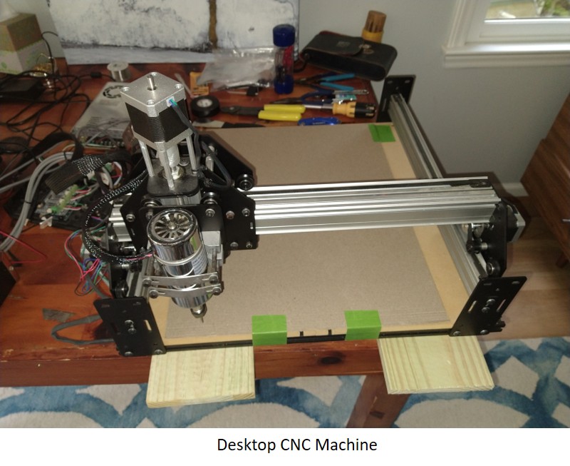
Print the curves and then paste them to a board to cut the shapes. If you have a CNC machine you can import the svg code directly into jscut to generate the gcode, or use gcmc.

But, there's a lot of wasted space in the plot generated by Octave. If you've ever tried to pack a bunch of stuff in the trunk of your car as you leave for vacation, or had to pack a trailer or rental truck full of household items for a move, you understand that efficient packing is key.
There's a math for that. But first,
P ≠ N P P \neq NP P=NP ... or Is It?
Many problems that we ask computers to solve are very easy, just tedious, which is why we like to have the computer do it. Adding a column of numbers, multiplying two large numbers together, sorting a set of words in lexicographic order, and searching for a string of words in a document are all the sorts of problems that computers do very well and quickly. If you ask a computer to sum n n n numbers and it takes t t t seconds, you'd expect that finding the sum of 2 n 2n 2n similar numbers would take about 2 t 2t 2t seconds. Problems that can be solved in time t = p ( n ) t = p(n) t=p(n) where p p p is a polynomial are said to be in class P P P, and there are efficient algorithms for finding the answers. The time required is called polynomial time because of the polynomial relationship between the number of inputs n n n and the processing time required, t t t.
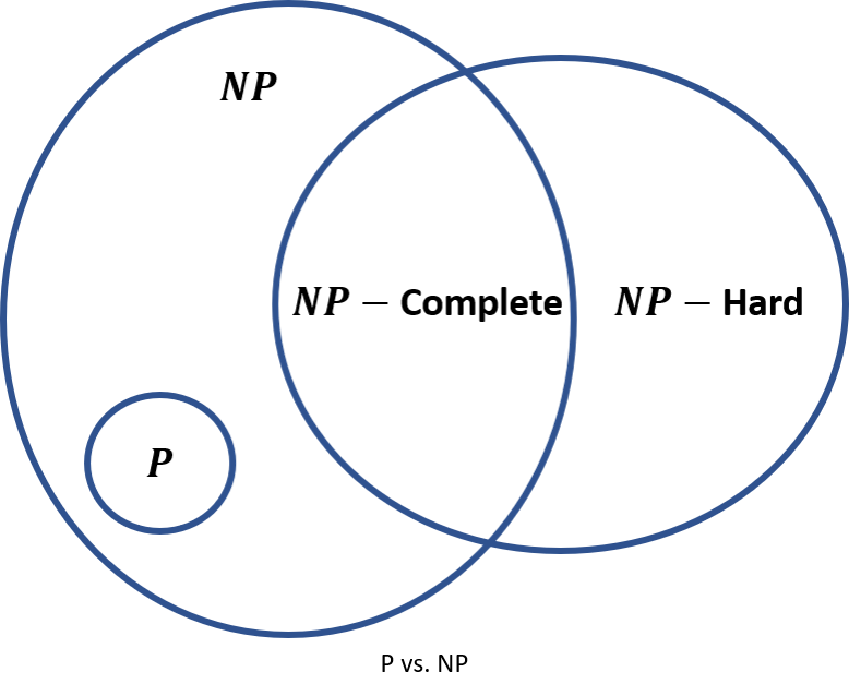
Problems in the class N P NP NP (nondeterministic polynomial) are easy to check in polynomial time, but nobody has found an algorithm to solve them in polynomial time. The nondeterministic part means that whatever state the computer is in at one point of the algorithm doesn't necessarily define what state will be next. KenKen puzzles are in N P NP NP because they're difficult to solve but easy to check. Every problem in P P P is also in N P NP NP because you can check the answer just by solving the problem again.
Why is there a question about P P P being equivalent to N P NP NP? Suppose you found some tricky algorithm that could quickly solve a KenKen puzzle in polynomial time. KenKen is thought to be in a sub-class called N P − NP- NP−complete which means that you can try every possible combination of solutions to see if one of them works (and it's easy to check if the solution is correct). It turns out that finding a polynomial time solution to an N P − NP- NP−complete problem would unlock solutions to all other N P NP NP problems. N P − NP- NP−hard problems are all the problems that are at least as hard as N P − NP- NP−complete problems:

The P P P vs N P NP NP problem is one of the seven Millennium Problems. Find an answer to any one of them and the Clay Mathematics Institute will give you one million dollars.

Bin Packer, Bin Packer, Pack Me A Bin

In a two-dimensional bin packing problem, we have several shapes (in our case section and bow/stern curves) that need to be optimally fitted into an area. Usually, the area is a rectangle, but that's not a requirement. The bin packing problem is in the class N P − NP- NP−hard meaning that there isn't a known algorithm that can optimally fill the bin in polynomial time. So the question we want to answer is, does there exist an order and orientation of K K K items with areas I j I_j Ij such that the sum of the sizes of items is less than or equal to the bin size B B B ( ∑ j = 1 K I j ≤ B ) (\sum_{j=1}^K I_j \leq B) (∑j=1KIj≤B)?
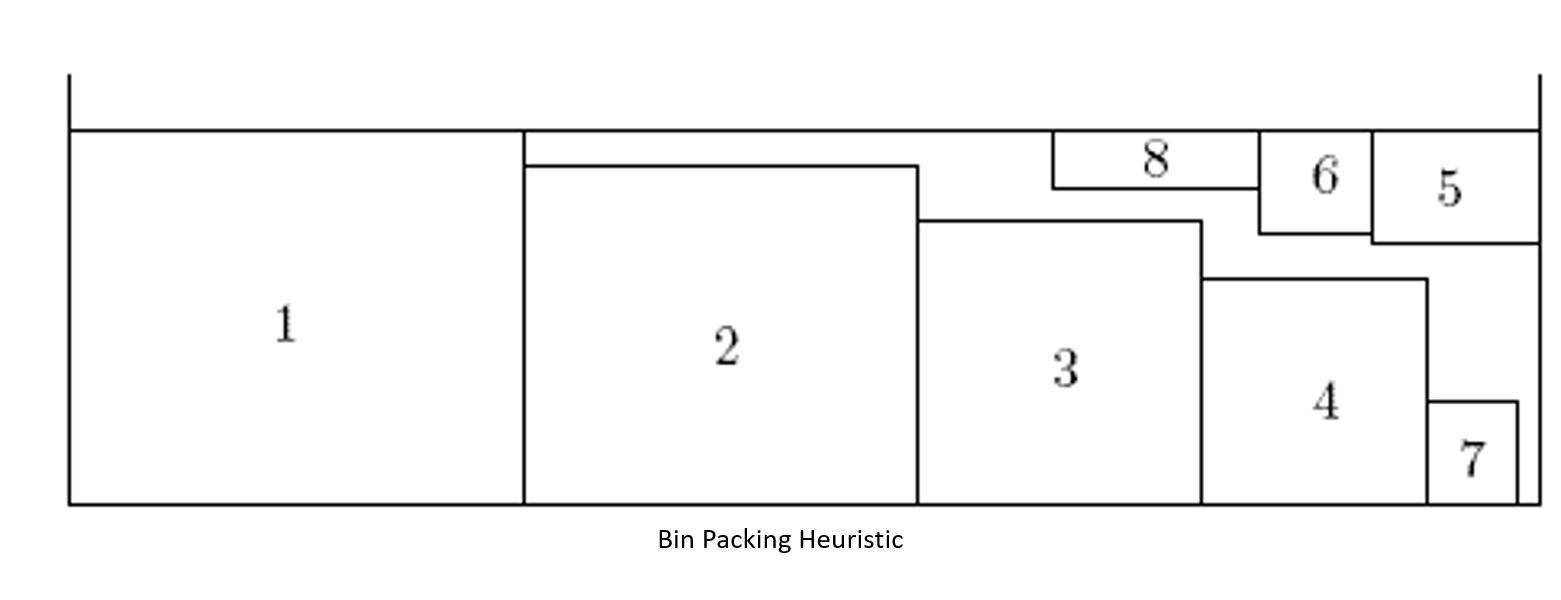
There are quite a few heuristic methods available. These algorithms choose the next item to be placed based on the size and orientation of the item, looking at the remaining available space and possible future items to pack. You could put the largest item in the lower-left corner of the bin, the next largest beside that one, and so on until you've filled items up to the right wall. Now work your way back towards the left side, still filling large to small, like this:

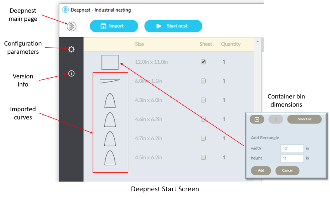
To read about other methods, see "Survey on two-dimensional packing". If you have just a few items to pack, you might try all possible arrangements, which is called the "brute force method". Implementing any of these algorithms might be considered "work", which we'd like to avoid. Instead, there's a very nice (free) nesting tool called Deepnest that handles the nesting for us. Download and install Deepnest, and then run it. You should see something like this (without the curves, yet):

Click on "Import" to begin selecting curves generated by Octave. When you've imported all of them (only 5 shown here) click on the "+" at the bottom of the page which will let you add a bounding rectangle that will become the container bin. Set the dimensions of the container and click "Add". This generates the rectangle shown at the top of the page. Under "Sheet", make sure that only the bin is checked to indicate which item is the container. In some cases, you may want to increase the quantities of some curves, which may be adjusted under the heading "Quantity".
You may also want to adjust the configuration parameters by clicking on the gear shown on the left side.

Hovering your cursor over any of the gray boxes brings up help information on the right side. Click on the Deepnest icon to return to the main page when done.
Next, click the "Start Nest" button which will switch to the nesting window,

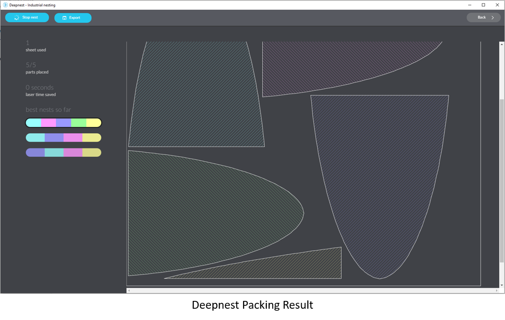
Nesting continues until you click "Stop nest" because the algorithm never knows if it's found the best possible solution. With just five pieces, it found a solution that gets all of them inside the bounding box, but there might be another way to do it that makes them fit more compactly. You'll have to run it until you think you've got a good enough fit. At that point, click on "Export" and save the nest file in .svg format.
Genetics
Deepnest uses a method called a Genetic Algorithm. Genetic algorithms mimic biological genetics by encoding information in strands of DNA, or what mathematicians call vectors. A vector is just an ordered list of numbers like, v = [ 1 , 5 , 7 , 2 , 42 , 8 ] v = \left[ 1, 5, 7, 2, 42, 8 \right] v=[1,5,7,2,42,8]. While working at the Institute for Advanced Study in Princeton, NJ, Alan Turing and Nils Barricelli used the IAS machine at night (when it wasn't being used to design the bomb) to study artificial life. Historian George Freeman wrote about the early work done building the first electronic computer at the IAS, "Turing's Cathedral", and gave a TED Talk, "The Birth of the Computer".
Genetic algorithms are a descendent of their early artificial life experiments, and use evolution to find near-optimal solutions to N P NP NP problems. A population of vectors is created randomly, the vectors are paired off to generate a new generation of offspring vectors and the best of breed are kept for subsequent generations.
Deepnest may be generating vectors where the numbers come in pairs. The first number is the piece number, and the second of the pair could indicate the orientation angle. The default number of orientation angles is 4 4 4, but you can change this in the configuration window.
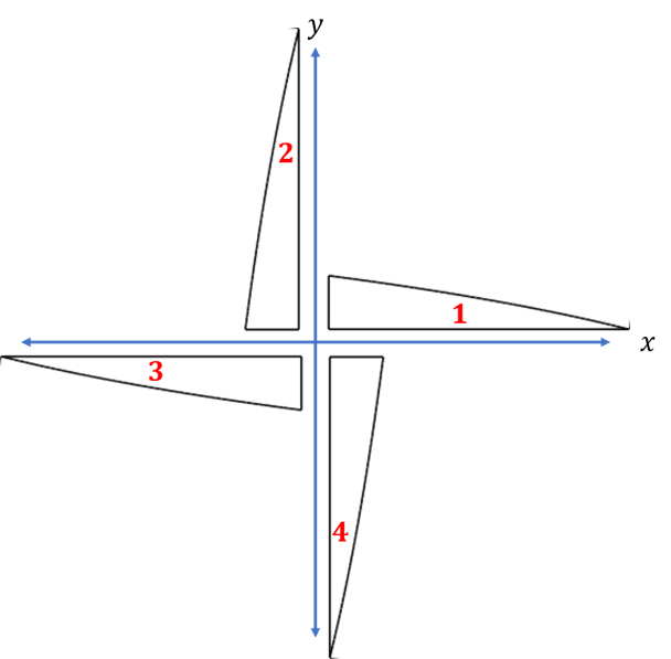
One way to encode the orientation would be to use a "1" if the orientation is on the positive x − x- x−axis, "2" for positive y y y, "3" for negative x x x and "4" for negative y y y,

A vector describing the order that items are placed in the bin and their orientation might be
v = [ 2 , 2 , 3 , 4 , 1 , 2 , 4 , 3 , 5 , 3 ] v = \left[2,2,3,4,1,2,4,3,5,3 \right] v=[2,2,3,4,1,2,4,3,5,3]meaning that the 2 n d 2^{nd} 2nd item would be placed first and it would be oriented along the y − y- y−axis, the 3 r d 3^{rd} 3rd item next along the negative y − y- y−axis and so on. By following the instructions in this DNA vector, the algorithm knows how and in what order to place each item. When it's done, the algorithm measures how much space was needed, and how many items were placed.
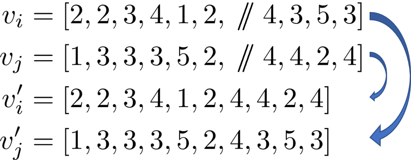
The genetic algorithm creates many of these DNA vectors and then randomly selects pairs to "breed" a new generation. Breeding is done by randomly selecting a point along the vector, snipping off the ends, and then swapping DNA.
Suppose you created a second vector with random placement order and orientations,
v i = [ 2 , 2 , 3 , 4 , 1 , 2 , 4 , 3 , 5 , 3 ] v j = [ 1 , 3 , 3 , 3 , 5 , 2 , 4 , 4 , 2 , 4 ] \begin{aligned} v_i &= \left[2,2,3,4,1,2,4,3,5,3 \right] \\ v_j &= \left[1,3,3,3,5,2,4,4,2,4 \right] \end{aligned} vivj=[2,2,3,4,1,2,4,3,5,3]=[1,3,3,3,5,2,4,4,2,4]Snip the ends off of v i v_i vi and v j v_j vj and swap the segments to form two new offspring vectors, v i ′ v'_i vi′ and v j ′ v'_j vj′,

In terms of the bin packing algorithm, this generates new packing rubrics that may be better than the original pair. In any case, we can try out both and pick the two best of v i , v i ′ , v j , v j ′ {v_i,v'_i,v_j,v'_j} vi,vi′,vj,vj′. With a large population of random DNA samples, the genetic algorithm rapidly converges to a very good solution.
There is a flaw with using this method for the bin packing algorithm because in almost every swap it's likely that you'll be packing two of some items, and none of some others. In v i ′ v'_i vi′ notice that the first item packed is 2 2 2 with orientation 2 2 2, but then 2 2 2 appears again at the end with orientation 4 4 4. If you want to pack one of every item, you could choose a permutation of the numbers 1 … n 1 \ldots n 1…n. There are n ! n! n! permutations and by choosing the next larger power of two, you could encode the permutation in binary.
In the example above, there are the eleven sections and bow/stern curves, and 11 ! = 39 , 916 , 800 11! = 39,916,800 11!=39,916,800. This would take 26 26 26 digits in binary, something like
v = [ 0 , 0 , 1 , 0 , 0 , 0 , 1 , 1 , 0 , 1 , 1 , 1 , 1 , 0 , 0 , 1 , 0 , 1 , 1 , 1 , 0 , 0 , 1 , 0 , 0 , 1 , 1 , 2 , 1 , 4 , 2 , 3 , 2 , 3 , 2 , 4 , 3 ] v = [0,0,1,0,0,0,1,1,0,1,1,1,1,0,0,1,0,1,1,1,0,0,1,0,0,1,1,2,1,4,2,3,2,3,2,4,3] v=[0,0,1,0,0,0,1,1,0,1,1,1,1,0,0,1,0,1,1,1,0,0,1,0,0,1,1,2,1,4,2,3,2,3,2,4,3]so the DNA vectors would become a bit longer, but not unmanageable. The first 26 26 26 digits ( 0 0 0s and 1 1 1s) form a unique binary encoding of a permutation of the numbers 1 − 11 1 - 11 1−11, while the last 11 11 11 numbers are randomly selected orientations. You have to create the binary encoding larger than 11 ! 11! 11!, and so some mappings won't work, but fortunately the coding for this problem is handled by Deepnest.
Greek Myths
For most applications of Deepnest, the items are visually distinguishable, but the section curves for this model are nearly identical and after they've been placed in the bin it's hard to tell one from another. One possible solution would be to include a unique number or letter with each item in .svg format. Another way would be to compare shapes since .svg files encode the locations of all points in the item. Of course, svg stands for "scalable vector graphics", so the encoded dimensions may change, and the orientation very likely is altered.
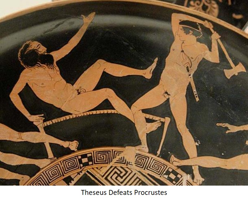
This is where Greek myths meet math geeks. In Greek mythology, Procrustes, the son of Poseidon, is described as an innkeeper and a bandit. Anyone who stayed at his inn had to fit the bed Procrustes provided, and nobody ever fit exactly. If the visitor was too short, Procrustes stretched him until he was long enough, and if he was too tall, his legs got cut off at the end of the bed. You might be better staying at M ο τ ϵ λ V I \Mu \omicron \tau \epsilon \lambda \; VI MοτϵλVI. In the end, Theseus fits Procrustes to his own bed.

For all myths Greek and Roman, check out Liv Albert's "Let's Talk About Myths, Baby!" podcast. That must be a typo. It should have been, "Let's Talk About Math, Baby!". Theseus may not have been so great either; episode V V V is "Theseus, Ruiner of Women & All Around Awful Person".
Anyway, the Procrustes method finds the best fit between two sets of points and can make correspondences between the initial set of curves provided to Deepnest and the completed packed set. If you can't get all of the curves on one sheet of paper or wood template, let Deepnest pack what it can, remove those items from the input set, and pack again until everything fits on several sheets.
Suppose you have two sets of points P = { p 1 , p 2 , … , p n } \mathcal{P} = \{p_1,p_2, \ldots, p_n \} P={p1,p2,…,pn} and Q = { q 1 , q 2 , … , q n } \mathcal{Q} = \{q_1,q_2, \ldots, q_n \} Q={q1,q2,…,qn} where P \mathcal{P} P are the input points before Deepnest packs them and Q \mathcal{Q} Q are the packed set. These points are in 2D, so each has coordinates p i = ( x i , y i ) p_i = (x_i,y_i) pi=(xi,yi). Deepnest shifts the set of points by some fixed distance t = ( t x , t y ) t = (t_x,t_y) t=(tx,ty) (called an affine transformation), scales the points by a constant σ \sigma σ and rotates them through an angle θ \theta θ. The rotation can be written as a matrix,
R = [ cos ( θ ) − sin ( θ ) sin ( θ ) cos ( θ ) ] . R = \begin{bmatrix} \cos(\theta) & -\sin(\theta) \\ \sin(\theta) & \cos(\theta) \end{bmatrix}. R=[cos(θ)sin(θ)−sin(θ)cos(θ)].Deepnest changes the scale of the bin and everything in it which is why we need the scaling factor, but we'll rescale both sets so we don't need to find σ \sigma σ. To find the best match between an input set P j \mathcal{P}_j Pj and nested set Q k \mathcal{Q}_k Qk we need to find the best fit between "visitor" and "bed". Mathematically, this means we need to find R R R and t t t that minimizes the function F F F,
F ( R , t ) = ∑ i = 1 n ∣ ∣ ( R p i + t ) − q i ∣ ∣ 2 . F(R,t) = \sum_{i=1}^n || (Rp_i + t) - q_i ||^2. F(R,t)=i=1∑n∣∣(Rpi+t)−qi∣∣2.The rotation matrix multiplies the x x x and y y y coordinates of point p i p_i pi by
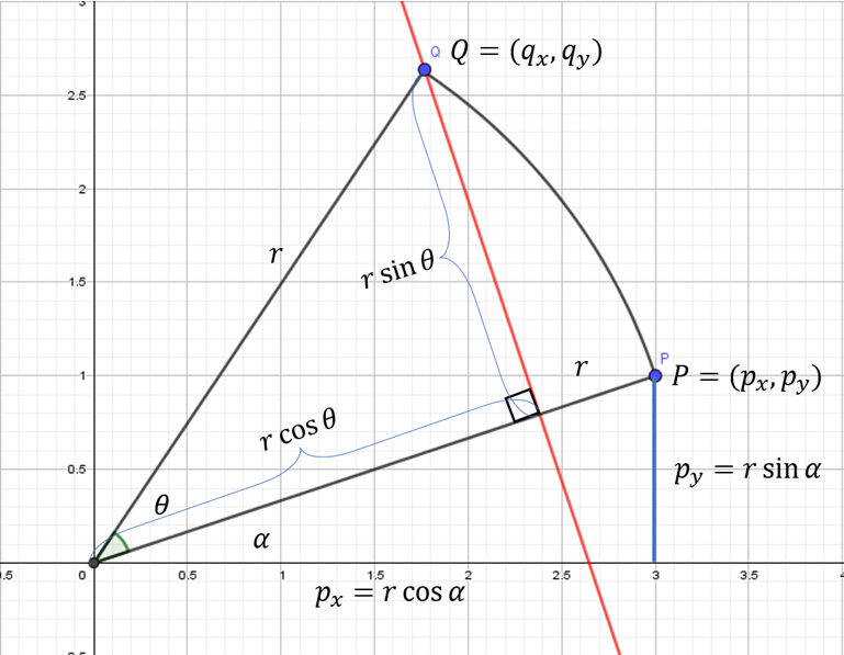
R p i = [ cos ( θ ) − sin ( θ ) sin ( θ ) cos ( θ ) ] [ x i y i ] = [ cos ( θ ) x i − sin ( θ ) y i sin ( θ ) x i + cos ( θ ) y i ] . Rp_i = \begin{bmatrix} \cos(\theta) & -\sin(\theta) \\ \sin(\theta) & \cos(\theta) \end{bmatrix} \begin{bmatrix}x_i \\ y_i \end{bmatrix} = \begin{bmatrix} \cos(\theta) x_i - \sin(\theta) y_i \\ \sin(\theta) x_i + \cos(\theta) y_i \end{bmatrix}. Rpi=[cos(θ)sin(θ)−sin(θ)cos(θ)][xiyi]=[cos(θ)xi−sin(θ)yisin(θ)xi+cos(θ)yi].In polar coordinates, p i = ( r cos α , r sin α ) p_i = (r \cos \alpha, r \sin \alpha) pi=(rcosα,rsinα), and to get to q i q_i qi we'll rotate about the origin by some angle θ \theta θ. Notice that the distance from the origin to both p i p_i pi and q i q_i qi is the constant r r r.

So the coordinates of Q Q Q are ( r cos ( α + θ ) , r sin ( α + θ ) ) (r \cos(\alpha + \theta), r \sin(\alpha + \theta)) (rcos(α+θ),rsin(α+θ)). Using the trigonometric identities,
cos ( α + θ ) = cos α cos θ − sin α sin θ sin ( α + θ ) = sin α cos θ + cos α sin θ \begin{aligned} \cos(\alpha + \theta) &= \cos \alpha \cos \theta - \sin \alpha \sin \theta \\ \sin(\alpha + \theta) &= \sin \alpha \cos \theta + \cos \alpha \sin \theta \end{aligned} cos(α+θ)sin(α+θ)=cosαcosθ−sinαsinθ=sinαcosθ+cosαsinθthe point
Q = ( r ( cos ( α + θ ) ) , r ( sin ( α + θ ) ) ) = ( r ( cos α cos θ − sin α sin θ ) , r ( sin α cos θ + cos α sin θ ) ) = ( r cos α cos θ − r sin α sin θ , r sin α cos θ + r cos α sin θ ) = ( p x cos θ − p y sin θ , p y cos θ + p x sin θ ) \begin{aligned} Q &= (r(\cos(\alpha + \theta)), r(\sin(\alpha + \theta))) \\ &= (r (\cos \alpha \cos \theta - \sin \alpha \sin \theta) , r (\sin \alpha \cos \theta + \cos \alpha \sin \theta) ) \\ &= ( r \cos \alpha \cos \theta - r \sin \alpha \sin \theta , r \sin \alpha \cos \theta + r \cos \alpha \sin \theta ) \\ &= (p_x \cos \theta - p_y \sin \theta , p_y \cos \theta + p_x \sin \theta ) \\ \end{aligned} Q=(r(cos(α+θ)),r(sin(α+θ)))=(r(cosαcosθ−sinαsinθ),r(sinαcosθ+cosαsinθ))=(rcosαcosθ−rsinαsinθ,rsinαcosθ+rcosαsinθ)=(pxcosθ−pysinθ,pycosθ+pxsinθ)which is the result of the matrix multiplication by R R R. The operator ∣ ∣ ⋅ ∣ ∣ || \cdot || ∣∣⋅∣∣ is the norm function, also known as the Euclidean Distance (Greeks again!), where
∣ ∣ p − q ∣ ∣ = ( p x − q x ) 2 + ( p y − q y ) 2 . ||p-q|| = \sqrt{(p_x - q_x)^2 + (p_y - q_y)^2}. ∣∣p−q∣∣=(px−qx)2+(py−qy)2.To find the affine translation t t t that minimizes F F F we can take the derivative and set it to 0 0 0,
0 = ∂ F ( R , t ) ∂ t = ∑ i = 1 n 2 ( R p i + t − q i ) = 2 t n + 2 R ∑ i = 1 n p i − 2 ∑ i = 1 n q i . \begin{aligned} 0 &= \frac{\partial F(R,t)}{\partial t} = \sum_{i=1}^n 2 (Rp_i + t - q_i) \\ &= 2tn + 2R \sum_{i=1}^n p_i - 2 \sum_{i=1}^n q_i. \\ \end{aligned} 0=∂t∂F(R,t)=i=1∑n2(Rpi+t−qi)=2tn+2Ri=1∑npi−2i=1∑nqi.Let p ˉ = 1 n ∑ i = 1 n p i \bar{p} = \frac{1}{n} \sum_{i=1}^n p_i pˉ=n1∑i=1npi and q ˉ = 1 n ∑ i = 1 n q i \bar{q} = \frac{1}{n} \sum_{i=1}^n q_i qˉ=n1∑i=1nqi be the centers of the points in P \mathcal{P} P and Q \mathcal{Q} Q. This means that t = q ˉ − R p ˉ t = \bar{q} - R \bar{p} t=qˉ−Rpˉ, so the optimal value of the affine transformation is just the difference between the centers, and substituting this value of t t t into F F F gives
F ( R , t ) = ∑ i = 1 n ∣ ∣ ( R p i + t ) − q i ∣ ∣ 2 = ∑ i = 1 n ∣ ∣ ( R p i + ( q ˉ − R p ˉ ) ) − q i ∣ ∣ 2 = ∑ i = 1 n ∣ ∣ R ( p i − p ˉ ) − ( q i − q ˉ ) ∣ ∣ 2 . \begin{aligned} F(R,t) &= \sum_{i=1}^n || (R p_i + t) - q_i ||^2 \\ &= \sum_{i=1}^n || (R p_i + (\bar{q} - R \bar{p})) - q_i ||^2 \\ &= \sum_{i=1}^n || R( p_i - \bar{p}) - (q_i - \bar{q}) ||^2. \end{aligned} F(R,t)=i=1∑n∣∣(Rpi+t)−qi∣∣2=i=1∑n∣∣(Rpi+(qˉ−Rpˉ))−qi∣∣2=i=1∑n∣∣R(pi−pˉ)−(qi−qˉ)∣∣2.To simplify, let's call p i ^ = p i − p ˉ \hat{p_i} = p_i - \bar{p} pi^=pi−pˉ and q i ^ = q i − q ˉ \hat{q_i} = q_i - \bar{q} qi^=qi−qˉ, in other words, the locations of the points after subtracting the centers. This puts the centers of both sets at the origin.
The norm squared can be written as
∣ ∣ ( R p i + t ) − q i ∣ ∣ 2 = ∣ ∣ R p i ^ − q i ^ ∣ ∣ 2 = ( R p i ^ − q i ^ ) T ( R p i ^ − q i ^ ) = ( p i ^ T R T − q i ^ T ) ( R p i ^ − q i ^ ) = p i ^ T R T R p i ^ − p i ^ T R T q i ^ − q i ^ T R p i ^ + q i ^ T q i ^ . \begin{aligned} || (R p_i + t) - q_i||^2 &= ||R \hat{p_i} - \hat{q_i} ||^2 \\ &= (R \hat{p_i} - \hat{q_i})^T(R \hat{p_i} - \hat{q_i}) = (\hat{p_i}^T R^T - \hat{q_i}^T )(R \hat{p_i} - \hat{q_i}) \\ &= \hat{p_i}^T R^T R \hat{p_i} - \hat{p_i}^T R^T \hat{q_i} - \hat{q_i}^T R \hat{p_i} + \hat{q_i}^T\hat{q_i}. \end{aligned} ∣∣(Rpi+t)−qi∣∣2=∣∣Rpi^−qi^∣∣2=(Rpi^−qi^)T(Rpi^−qi^)=(pi^TRT−qi^T)(Rpi^−qi^)=pi^TRTRpi^−pi^TRTqi^−qi^TRpi^+qi^Tqi^.Since R R R is a rotation, the product R T R = I R^TR = I RTR=I, the identity matrix (all ones on the diagonal and zeros elsewhere), so p i ^ T R T R p i ^ = p i ^ T p i ^ \hat{p_i}^T R^T R \hat{p_i} = \hat{p_i}^T \hat{p_i} pi^TRTRpi^=pi^Tpi^, and since p i ^ T R T q i ^ \hat{p_i}^T R^T \hat{q_i} pi^TRTqi^ is a scalar (number) taking the transpose doesn't change the value, so p i ^ T R T q i ^ = q i ^ T R p i ^ \hat{p_i}^T R^T \hat{q_i} = \hat{q_i}^T R \hat{p_i} pi^TRTqi^=qi^TRpi^. Now, the first and last terms don't have R R R in them, so minimizing this with respect to R R R is equivalent to finding the minimum of − 2 q i ^ T R p i ^ -2 \hat{q_i}^T R \hat{p_i} −2qi^TRpi^ over all i i i,
min ∑ i = 1 n ( − 2 q i ^ T R p i ^ ) = min ( − 2 ∑ i = 1 n q i ^ T R p i ^ ) = max ∑ i = 1 n ( q i ^ T R p i ^ ) . \min \sum_{i=1}^n \left( -2 \hat{q_i}^T R \hat{p_i} \right) = \min \left(-2 \sum_{i=1}^n \hat{q_i}^T R \hat{p_i} \right) = \max \sum_{i=1}^n \left( \hat{q_i}^T R \hat{p_i} \right). mini=1∑n(−2qi^TRpi^)=min(−2i=1∑nqi^TRpi^)=maxi=1∑n(qi^TRpi^).The coefficient − 2 -2 −2 can be ignored because it only changes the value of the minimum, but removing the minus sign changes a minimum to a maximum.
Let's call P ^ \hat{\mathcal{P}} P^ the 2 × n 2 \times n 2×n array of translated points p i ^ = ( p x i , p y i ) \hat{p_i} = (p_x^i,p_y^i) pi^=(pxi,pyi) and Q ^ \hat{\mathcal{Q}} Q^ the equivalent 2 × n 2 \times n 2×n array for q i ^ = ( q x i , q y i ) \hat{q_i} = (q_x^i,q_y^i) qi^=(qxi,qyi). Then if you multiply Q ^ T R P ^ \hat{\mathcal{Q}}^T R \hat{\mathcal{P}} Q^TRP^ the result is an n × n n \times n n×n array, but along the diagonal are the terms q i ^ T R p i ^ \hat{q_i}^T R \hat{p_i} qi^TRpi^. Adding up all of the elements of the diagonal of a matrix is called the trace ( tr ) (\text{tr}) (tr) of the matrix, so
∑ i = 1 n ( q i ^ T R p i ^ ) = tr ( Q ^ T R P ^ ) . \sum_{i=1}^n \left( \hat{q_i}^T R \hat{p_i} \right) = \text{tr} \left( \hat{\mathcal{Q}}^T R \hat{\mathcal{P}} \right). i=1∑n(qi^TRpi^)=tr(Q^TRP^).By itself, this doesn't seem that it helps much but the trace operator has properties that we can use, one of them being that for any pair of compatible matrices A A A and B B B, tr ( A B ) = tr ( B A ) \text{tr}(AB) = \text{tr}(BA) tr(AB)=tr(BA). For the arrays here, this means that
tr ( Q ^ T ( R P ) ^ ) = tr ( ( R P ^ ) Q ^ T ) . \text{tr} \left( \hat{\mathcal{Q}}^T (R \hat{\mathcal{P})} \right) = \text{tr} \left( (R \hat{\mathcal{P}}) \hat{\mathcal{Q}}^T \right). tr(Q^T(RP)^)=tr((RP^)Q^T).Next, let S = P ^ Q ^ T \mathcal{S} = \hat{\mathcal{P}}\hat{\mathcal{Q}}^T S=P^Q^T. Since P ^ \hat{\mathcal{P}} P^ is a 2 × n 2 \times n 2×n array and Q ^ T \hat{\mathcal{Q}}^T Q^T is n × 2 n \times 2 n×2 then S \mathcal{S} S is 2 × 2 2 \times 2 2×2. Using the Singular Value Decomposition (svd) we can write S \mathcal{S} S as
S = U Σ V T . \mathcal{S} = U \Sigma V^T. S=UΣVT.The matrices U U U and V V V are unitary meaning that if you multiply them by their conjugate transposes you get the identity matrix. The matrix in the middle, Σ \Sigma Σ is diagonal and the elements on the diagonal are called the singular values. Substituting S \mathcal{S} S into the equation for the trace,
tr ( R P ^ Q ^ T ) = tr ( R S ) = tr ( R U Σ V T ) = tr ( Σ V T R U ) . \text{tr} \left( R \hat{\mathcal{P}} \hat{\mathcal{Q}}^T \right) = \text{tr}(R \mathcal{S}) = \text{tr}(R U \Sigma V^T) = \text{tr}(\Sigma V^T R U). tr(RP^Q^T)=tr(RS)=tr(RUΣVT)=tr(ΣVTRU).Since U , V U,V U,V and R R R are all orthogonal matrices then the product M = V T R U M = V^T R U M=VTRU is also orthogonal, so columns of M M M are 2 × 1 2 \times 1 2×1 orthonormal vectors and all of the entries of M M M are less than or equal to one, meaning
1 = m j T m j = ∑ i = 1 2 m i j 2 ⟹ m i j 2 ≤ 1 ⟹ ∣ m i j ∣ ≤ 1. 1 = m_j^Tm_j = \sum_{i=1}^2 m_{ij}^2 \implies m_{ij}^2 \leq 1 \implies |m_{ij}| \leq 1. 1=mjTmj=i=1∑2mij2⟹mij2≤1⟹∣mij∣≤1.Since Σ V T R U = Σ M \Sigma V^T R U = \Sigma M ΣVTRU=ΣM we can bound the trace of Σ M \Sigma M ΣM as
tr ( Σ M ) = ∑ i = 1 2 σ i m i i ≤ ∑ i = 1 2 σ i . \text{tr}(\Sigma M) = \sum_{i=1}^2 \sigma_i m_{ii} \leq \sum_{i=1}^2 \sigma_i. tr(ΣM)=i=1∑2σimii≤i=1∑2σi.To maximize tr ( Σ M ) \text{tr}(\Sigma M) tr(ΣM) each entry m i i m_{ii} mii must be 1 1 1 which means that M M M is the identity matrix. In other words,
I = M = V T R U ⟹ V = R U ⟹ R = V U T . I = M = V^T R U \implies V = RU \implies R = VU^T. I=M=VTRU⟹V=RU⟹R=VUT.We can get the rotation matrix R R R that maps P ^ \hat{\mathcal{P}} P^ into Q ^ \hat{\mathcal{Q}} Q^ by calculating S = P ^ Q ^ T \mathcal{S} = \hat{\mathcal{P}}\hat{\mathcal{Q}}^T S=P^Q^T, computing the svd of S = U Σ V T \mathcal{S} = U \Sigma V^T S=UΣVT, and then getting R = V U T R = VU^T R=VUT. Very simple!
This is the basis of the Procrustes method when P \mathcal{P} P and Q \mathcal{Q} Q have the same number of points. In many cases, points will be missing from one set or the other and the Procrustes method needs to be modified. One way to do this is with The Softassign Procrustes Matching Algorithm.
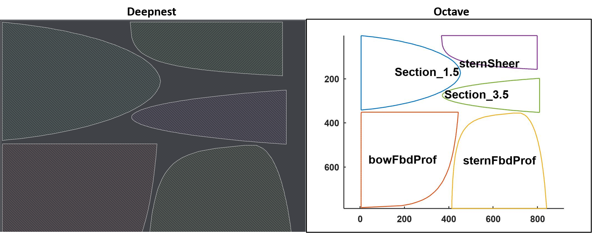
The Octave function idNestObjects.m reads in the set of .svg files generated by bez2svg.m and the file of nested objects from Deepnest, makes the corresponding identifications and plots the curves with their identifying file names. On the left is the result of the Deepnest packing algorithm and on the right is the identification by Octave:

The Recipe
To build a model boat using foam and a hot wire cutter, follow these steps:
- Draw the hull lines (sheer, freeboard, profile, sections, homotopy) as described in Yacht Design with Mathematics. You can use the online version of Geogebra if you don't want to download it.
- Using the Octave function BezierHull.m, generate the lines structure:
BezStruct = BezierHull(<fName>);. - Make a new directory for svg files, then run bez2svg.m:
bez2svg(BezStruct,<svgDir>);. - Install Deepnest.io, load the svg files, and begin packing. Stop when a good solution is found, and save the nested svg file.
- Identify the parts using idNestObjects.m:
idNestObjects(<svgDir>,<NestFile>);. Save the image with ID'd objects so you can match it to the nested svg file later. You'll need the Octave/Matlab function v2struct.m which is called fromidNestObjects. Delete curves in the input list in Deepnest and repeat until all of the objects have been nested. Inkscape is useful for plotting svg image files. - Print the curves, cut them out, and attach them to the foam blocks. Build the hot wire foam cutter, and begin cutting out the hull.
If anyone asks, you're not making a toy boat out of old pieces of Styrofoam you threw in the garage for some project, you're ...
Applying a genetic algorithm to determine a heuristically optimal solution to an N P − NP- NP−hard bin packing method of orthogonal sections through a C ∞ C^\infty C∞ smooth S 2 \mathbb{S}^2 S2 manifold generated from Bezier polynomials and homotopies, and then applying the Procrustes method to form a bijective mapping between pre and post-packed coordinate sets. It sounds a lot more important that way.
Image credits
-
Hero: An image of “kottabos with a pole” getting set up. The History of Ancient Greece Podcast, Ryan Stitt
-
Hot Wire Foam Cutter, Cutting the Foam: Hot Wire Foam Cutting. Flite Test, Apr 30, 2013.
-
Doctor Evil: Austin Powers Doctor Evil GIF. Uploaded: 09/13/2015.
-
Bin Packing with Dog: Black and brown Dachshund standing in box. Erda Estremera Unsplash, Mar 2, 2018.
-
Theseus Defeats Procrustes: Procrustes. Intermedia, Zuraband, Mar. 25, 2016.
Code and Software
BezierHull.m - Octave functions for generating Bezier yacht hull curves using Letcher's method: BezierHull, symBezFunc, funcSolve, write2DELFTship, scale
bez2svg.m - Converts curves in BezStruct to svg format: bez2svg, func2Coords, section_at_x, funcSolve, pts2svg, disperse
idNestObjects.m - Returns a list of objects found in a nest generated by Deepnest.io: idNestObjects, svg2paths, normPaths, plotNested, vnorm
- Deepnest - is an open source nesting application, great for laser cutters, plasma cutters, and other CNC machines.
- Octave - GNU Octave is a high-level language, primarily intended for numerical computations. It provides a convenient command line interface for solving linear and nonlinear problems numerically, and for performing other numerical experiments using a language that is mostly compatible with Matlab.
- Geogebra - GeoGebra is dynamic mathematics software for all levels of education that brings together geometry, algebra, spreadsheets, graphing, statistics and calculus in one easy-to-use package.
- Inkscape - Inkscape is a Free and open source vector graphics editor for GNU/Linux, Windows and macOS. It offers a rich set of features and is widely used for both artistic and technical illustrations such as cartoons, clip art, logos, typography, diagramming and flowcharting. It uses vector graphics to allow for sharp printouts and renderings at unlimited resolution and is not bound to a fixed number of pixels like raster graphics. Inkscape uses the standardized SVG file format as its main format, which is supported by many other applications including web browsers.
- DELFTship - Yacht visual hull form modeler.
- LibreOffice - LibreOffice is a powerful and free office suite, with a clean interface and feature-rich tools help you unleash your creativity and enhance your productivity.
References and further reading
- Hot Wire Foam Cutting, Flite Test, Flite Test Blog, 30 Apr 2013.
- JA 37 Viggen Scratch Build, Flite Test, Flite Test Blog, 07 Sep 2021.
- Survey on Two-Dimensional Packing, E.P. Anagnostopoulos, University of Liverpool, Date Unknown.
- Deepnest - Open Source Nesting Software, Jack Qiao, Deepnest.io, 07 Sep 2021.
- The Softassign Procrustes Matching Algorithm, Anand Rangarajan et al., University of Florida, Date Unknown.
- Understanding Singular Value Decomposition and Its Application in Data Science, Aditi Roy, Towards Data Science, 12 Mar 2018.
📬 Subscribe and stay in the loop. · Email · GitHub · Forum · Facebook
© 2020 – 2025 Jan De Wilde & John Peach
